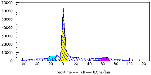
In addition to the kinematics cuts and other, track based cuts applied to our data, we also have the more fundamental cuts applied to the raw nDet hits. There are two such cuts routinely applied to the data prior to tracking: a cut (window) on the corrected meantime of the individual hits and a cut (minimum) on the energy deposited in the nDet bar by the hit.
While we want to determine the background contamination in our tracks, this cannot be accomplished if we discard the hits that are outside the nDet--HMS coincidence time window. We therefore need to modify this meantime requirement on the hits we create tracks from.
This could be accomplished by simply removing this requirement. However, this creates a complication: Our normal tracking prcedure only allows a certain window of hit meantimes for those hits actually considered for tracking. More importantly, this meantime window is quite close to the window of track times we allow. Also, any two hits that are within +/-10ns of each other have a realistic probability of being used in the same track -- excluded only via some fairly generous geometry requirements or the meantime window boundary.
This means that removing this boundary may change the set of hits that together define a given track. Since the time of the track is given by one of the hits, the one closest to the target and lowest to the ground, the time attributed to the track might change as well. The track is then at a different time (t') than it used to be before the hit meantime window was removed (t0). This means we can no longer associate it with the tracks that remain at the time this track used to be at. Similarly, other tracks are now given a track time of t0 although they used to be later (or earlier?).
What it all boils down is this: removing the meantime window cut results in a changed time distribution of the resultant tracks, not merely an addition of new tracks. We can therefore not compare the "background tracks" obtained without a meantime window and the "background diluted coincidence tracks" ontained with the meantime cut.
If we instead shift the meantime window, the relative relationship between the hits inside the window and those outside is unchanged. By definition, the background we are after is isotropic and thus only this relative relationship is relevant. We can now be confident in the assumption that the background tracks have the same distribution inside our nominal meantime window as they do in our shifted cut, and apply this correction to our data.
|
Background Rate and Dilution Correction
Here now are the results of analyzing the data with the various definition of the hit meantime window. The plot shows the time spectrum of the tracks abtained seperately for early, late and nominal time windows, as well as those for no meantime cut. The lower (apparent) yield obtained without a hit time cut is apparent throughout.

|
Below are the details of the study, for each run in the test sample. Included are the track count per time bin and summed over the entire track time window, for all hits and for standard proton and neutron definitions. We also determined the rate of tracks for each meantime window, normalized to a beam current of 100nA, and the ratio between the early background and the nominal rate.
| ||||||||||||||||||||||||||||||||||||||||||||||||||||||||||||||||||||||||||||||||||||||||||||||||||||||||||||||||||||||||||||||||||||||||||||||||||||||
We are using the "early" levels for the background rate determination because the "late" level is ill-defined (it is included here only for completeness). The actual hit time used to define the track time is the corrected meantime but only after the hit time has been extrapolated back to plane 3. This plot shows how this adjustment distorts the track time. For early hits this is not an issue because the adjustment is then very small (actually, it's also negative and the significant point is that the time is not that different from 0). The adjustment increases with time and also with plane number. A portion of our background tracks in the "late" peak is thus mapped to earlier times, reducing the rate. Without accounting for the plane the hit(s) are in, we cannot correct for this effect. Besides, the late tail is bound to contain some non-noise hits, a dilution we do not have to consider in the "early" case.
| ||||||||||||||||||||||||||||||||||||||||||||||||||||||||||||||||||||||||||||||||||||||||||||||||||||||||||||||||||||||||||||||||||||||||||||||||||||||
Our discussion so far has been based on the assumption that a hit is either composed of background hits or of "good" coincidence hits. In the actual event processing, we cannot distinguish between noise and "good" hits (otherwise this exercise would be superfluous) and we therefore have to allow for both types of hits to be used in the creation of a single track. This leaves us with a rather fundamental decision: do we discard these mixed tracks or do we include them in the "good" data set?
In either case, we need to quantify the intermixing. An initial guess might be to scale the number of background tracks according to the ratio of background hits to the total number of hits in the coincidence peak (i.e. background plus "good"). An excess would then be attributable to the intermixing of hits. It turns out, however, that the noise level is sufficiently low for the non-random nature of the "good" tracks to dominate the scaled isotropic noise and the excess is in the opposite direction from the expected.
A different approach is therefore needed. We know the number of hits due to noise, we know how many tracks these noise hits ought to create, and we know how many total hits and tracks there are. We also know that the "good" hits are more "efficient" in the track creation.
What now? FYI, some plots:
- number of track-starts per plane (p and n, nominal and late)
- number of tracks per bar, nominal (p and n, by plane)
- number of tracks per bar, early (p and n, by plane)
- hits per track (p and n, nominal and late)
- number of tracks per HMS event
Pulse Fiction
credit for this approach goes to Yury G. Kolomensky (as far as I know)To resolve this issue, we can try a different approach. If we somehow can controll the number of background hits, we can determine how the number of tracks is affected. Since we already know the number of background hits, this might allow us to determine the number of genuine background tracks in our data set. Since our TDCs only allow one hit per event, any channel that registers an early hit cannot contribute later. We can therefore use the earlier hits to create the controlled increase in background.
The results of mapping all the hits from the early meantime window into the nominal interval, by shifting the hit time consistently by 18ns, are shown below. Note that the quoted run averages are not the histogram average, as this would be incorrect; instead, the average given is the result of doing the background extraction with the sum of track in the allowed track time interval. The effect is that the bins where there are many good tracks weigh more significant than those with fewer tracks, regardless of the difference between good and noise hits.
| Bkgnd = | noise data |
= | extra - nominal nominal - (extra - nominal) |
The procedure is easy to understand if you look at the hit distribution plot at the top of this page. The hits in the early time window are unformly shifted until the entire early window exctaly overlays the nominal meantime window, but only the hits in the early window. The resultant distribution would have an empty gap in the early window. These hits now contribute to the track creation. They will either add to tracks that existed anyway (when only the actaul hits are used) or they will make tracks of their own.
 |
By comparing the results with those obtained using nomnial reconstruction, we can conclusively determine the impact of adding these hits. Here are two sample plots detailing the results for run 41505, the same one providing the above hit distribution. This overview plot shows the total number of tracks per 0.1ns bin of track time. In blue are the distributions abtained by using either the nominal or the early meantime window seperately, and in yellow the additional tracks created after the early hits have been mapped into the nominal hit meantime window. |
| A more detailed plot again compares the track time spectrum for nominal and pulse fiction hit meantimes (left column), and also shows the fractional difference between nominal and pulse fiction tracks (difference divided by nominal). These plots are provided for the entire, uncut track spectrum and for standard proton and neutron definitions. Also indicated in the relative plots is the average fractional difference. Remember that the quoted average is wheighed by the number of tracks in the respective time bin; at least that's effectively what happens -- see note at the top of this section. For the neutrons, we also extrapolated back to find the difference between nominal and clean track spectra and this results in the indicated background level. |
 |
To date, we have no explanation for the fact that the number of proton tracks decreases when the additional hits are added. Since each coincidence event only contains one track, it cannot be explained by the new hits merging multiple tracks into one. Further investigations are underway.
The results for the same set of runs used in the other background studies are tabulated below; the same data are also summarized in this plot, which shows the fractional contamination in the neutron data for all the examined runs.
| ||||||||||||||||||||||||||||||||||||||||||||||||||||||||||||||||||||||||||||||||||||||||
The remaining question is whether the noise that is already present anyway, without us adding it artificially, has the exact same impact, relative to the number of good tracks. To answer this question, we are replaying a subset of these runs with two seperate early windows mapped into the nominal hit menatime interval. If the number of background tracks increases linearly with the increase in noise hits, then we can simply extrapolate backwards, removing the flat rate of background hits, to find the true background contamination.
A systematic check on the dependence on the exact location of the early meantime window, is also under way.
In Progress.
Background Asymmetry and Correction
The background asymmetry, however, is a different story. Here, we do not actually care about the exact time of the (background) tracks, as long as both beam helicities are treated equally. If we are then looking at a time where the hits that might have entered into the creation of the track are guaranteed to be background hits, the resulting track asymmetry is bound to be representative of the background.
| ||||||||||||||||||||||||||||||||||||||||||||||||||||||||||||||||||||||
The general consensus appears to be that this result is sufficiently consistent with zero for no correction to be required...

