Difference between revisions of "Elong-13-09-27"
From HallCWiki
Jump to navigationJump to search| (2 intermediate revisions by the same user not shown) | |||
| Line 4: | Line 4: | ||
{| class="wikitable" style="text-align:center; border-collapse:collapse;" border="1" | {| class="wikitable" style="text-align:center; border-collapse:collapse;" border="1" | ||
| − | ! | + | ! $b_1^{\mathrm{DIS}}$ !! $b_1^{\mathrm{QE}}$ !! $A_{zz}$ |
|- | |- | ||
| [[Image:2013-09-27-b1-dis.png|500px]] || [[Image:2013-09-27-b1-qe.png|500px]] || [[Image:2013-09-27-Azz.png|500px]] | | [[Image:2013-09-27-b1-dis.png|500px]] || [[Image:2013-09-27-b1-qe.png|500px]] || [[Image:2013-09-27-Azz.png|500px]] | ||
| Line 14: | Line 14: | ||
[[Image:2013-09-27-Azz-full-range.png|350px]] [[Image:2013-09-27-q2-full-range.png|345px]] | [[Image:2013-09-27-Azz-full-range.png|350px]] [[Image:2013-09-27-q2-full-range.png|345px]] | ||
| − | |||
| − | |||
| − | |||
| − | |||
| − | |||
| − | |||
| − | |||
--[[User:Ellie|E. Long]] 21:20, 27 September 2013 (UTC) | --[[User:Ellie|E. Long]] 21:20, 27 September 2013 (UTC) | ||
Latest revision as of 13:55, 18 October 2023
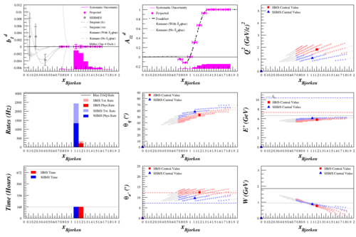
0.09<x<1.85 Azz Measurement
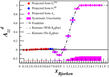
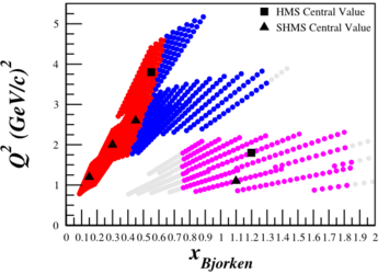
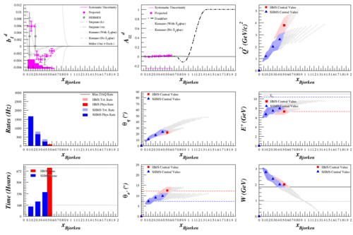
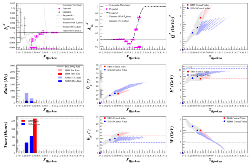
If we move forward with the new Azz measurement and combine it with the data that we'll get from b1, we'll have measurements of Azz over a large x range.
| $b_1^{\mathrm{DIS}}$ | $b_1^{\mathrm{QE}}$ | $A_{zz}$ |
|---|---|---|
 |
 |
|
If we combine all three of these into a single plot, it shows the entire range.
--E. Long 21:20, 27 September 2013 (UTC)
