Difference between revisions of "Elong-15-02-26"
| (One intermediate revision by the same user not shown) | |||
| Line 9: | Line 9: | ||
==2012 World Data== | ==2012 World Data== | ||
| − | I talked with Ron Gilman, who has kindly passed on world data from 2012 as summarized in [http://iopscience.iop.org/0034-4885/75/8/086301/ Holt & Gilman (2012)]. In particular, he noted that low Q^2 t20 measurements could be invaluable for confirming that we understand the target tensor polarization, as | + | I talked with Ron Gilman, who has kindly passed on world data from 2012 as summarized in [http://iopscience.iop.org/0034-4885/75/8/086301/ Holt & Gilman (2012)]. In particular, he noted that low Q^2 t20 measurements could be invaluable for confirming that we understand the target tensor polarization, as $t_{20}$ is best known experimentally and theoretically in the 0<Q<sup>2</sup><0.16 (GeV/c)<sup>2</sup> region, which coincides with what will likely be the "cheapest" points. |
[[Image:2015-02-26-d-2012-data.png]] | [[Image:2015-02-26-d-2012-data.png]] | ||
| Line 15: | Line 15: | ||
==Long Parameterization== | ==Long Parameterization== | ||
| − | Donal sent me parameterizations of A and B that M. Petratos put together, of the form | + | Donal sent me parameterizations of A and B that M. Petratos put together, of the form $F=10^{([0]+[1]*x+[2]*x^2)}$ where x=Q^2 and F=A or B. |
For A, he used [0]=-2.5275, [1]=-1.5704, [2]=0.09667. | For A, he used [0]=-2.5275, [1]=-1.5704, [2]=0.09667. | ||
| Line 27: | Line 27: | ||
For A, I used the equation | For A, I used the equation | ||
| − | + | $A=10^{([0]+[1]*x+[2]*x^2+[3]*x^3)}+10^{(-2.68235-1.47849*x+0.0782541*x^2)}$ | |
where x=Q^2 and [0]=-1.85931e-02, [1]=-1.37215e+01, [2]=3.23622e+01, [3]=-4.29740e+01. The reason I used two added functions is due to there being a "kink" region around Q^2~0.6. | where x=Q^2 and [0]=-1.85931e-02, [1]=-1.37215e+01, [2]=3.23622e+01, [3]=-4.29740e+01. The reason I used two added functions is due to there being a "kink" region around Q^2~0.6. | ||
| Line 34: | Line 34: | ||
[[Image:2015-02-26-A_fit.png]] [[Image:2015-02-26-B_fit.png]] | [[Image:2015-02-26-A_fit.png]] [[Image:2015-02-26-B_fit.png]] | ||
| − | |||
| − | |||
Very very preliminary t20 fit: | Very very preliminary t20 fit: | ||
[[Image:2015-02-26-t20_basic_fit.png|400px]] (Note: Extremely preliminary, overly simplistic fit) | [[Image:2015-02-26-t20_basic_fit.png|400px]] (Note: Extremely preliminary, overly simplistic fit) | ||
Latest revision as of 14:29, 18 October 2023
Deuteron Form Factors Parameterization
Abbot Parameterization
Best as I've found, the most recent deuteron form factor parameterization comes from Abbot, et al (2000), who give parameter equations but not the parameters. They are also using world data from 2001, which is missing a number of new points.
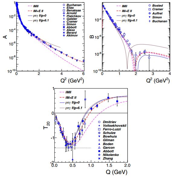
2012 World Data
I talked with Ron Gilman, who has kindly passed on world data from 2012 as summarized in Holt & Gilman (2012). In particular, he noted that low Q^2 t20 measurements could be invaluable for confirming that we understand the target tensor polarization, as $t_{20}$ is best known experimentally and theoretically in the 0<Q2<0.16 (GeV/c)2 region, which coincides with what will likely be the "cheapest" points.
Long Parameterization
Donal sent me parameterizations of A and B that M. Petratos put together, of the form $F=10^{([0]+[1]*x+[2]*x^2)}$ where x=Q^2 and F=A or B.
For A, he used [0]=-2.5275, [1]=-1.5704, [2]=0.09667.
For B, he used [0]=-2.1870, [1]=-3.4066, [2]=0.44380.
I calculated the chi^2/ndf of both of these, and created new parameters for the 2012 world data.
For B, I used the same form as Petratos above but with [0]=-2.26938, [1]=-3.18194, [2]=0.147926
For A, I used the equation
$A=10^{([0]+[1]*x+[2]*x^2+[3]*x^3)}+10^{(-2.68235-1.47849*x+0.0782541*x^2)}$
where x=Q^2 and [0]=-1.85931e-02, [1]=-1.37215e+01, [2]=3.23622e+01, [3]=-4.29740e+01. The reason I used two added functions is due to there being a "kink" region around Q^2~0.6.
Results from both are shown below.
Very very preliminary t20 fit:


