Difference between revisions of "Elong-14-04-16"
| (22 intermediate revisions by the same user not shown) | |||
| Line 1: | Line 1: | ||
| + | =Deuteron Polarization= | ||
| + | |||
| + | Being a spin-1 particle, the deuteron has three spin sub-states that can be filled: $m_J=+1,~m_J=0,~m_J=-1$. For a given quantity of deuterons, the polarization is measured based on the population $p_m$ in each substate. The population is defined as | ||
| + | |||
| + | $p_m=\frac{N_m}{N_1+N_0+N_{-1}}$ | ||
| + | |||
| + | where $N_m$ is the number of deuterons in a given substate. In a system of pure deuterons, the normalization of the populations is | ||
| + | |||
| + | $p_1+p_0+p_{-1}=1$. | ||
| + | |||
| + | |||
| + | |||
| + | Vector polarization depends only on the $m_J=\pm 1$ populations, such that | ||
| + | |||
| + | $P_z = p_1 - p_{-1}~$. | ||
| + | |||
| + | It has a range of $-1<P_z<1~$. | ||
| + | |||
| + | If the $m_1$ state is filled, then $p_1=1,~p_{-1}=0,~p_0=0$ and $P_z=1~$. | ||
| + | |||
| + | If the $m_{-1}$ state is filled, then $p_1=0,~p_{-1}=1,~p_0=0$ and $P_z=-1~$. | ||
| + | |||
| + | If the $m_0$ state is filled, then $p_1=0,~p_{-1}=0,~p_0=1$ and $P_z=0~$. | ||
| + | |||
| + | |||
| + | |||
| + | Tensor polarization depends on the combined $m_J=\pm 1$ populations, as well as the $m_J=0$ population such that | ||
| + | |||
| + | $P_{zz} = (p_1 + p_{-1}) - 2p_0~$. | ||
| + | |||
| + | It has a range of $-2<P_{zz}<1~$. | ||
| + | |||
| + | If the $m_1$ and $m_{-1}$ states are filled, then $(p_1 + p_{-1})=1,~p_0=0$ and $P_{zz}=1~$. | ||
| + | |||
| + | If the combined $m_1$ and $m_{-1}$ states equal the $m_0$ state, then $(p_1+p_{-1})=0.5,~p_0=0.5$ and $P_{zz}=-0.5~$ | ||
| + | |||
| + | If the $m_0$ state is filled, then $(p_1 + p_{-1})=0,~p_0=1$ and $P_{zz}=-2~$. | ||
| + | |||
| + | [[Image:2014-08-21-Pzz-vs-m0.png|600px]] | ||
| + | |||
| + | Or, in terms of an overly-simplistic animation, | ||
| + | |||
| + | [[Image:2014-08-22-Pzz-animation-food.gif|300px]] | ||
| + | |||
=Deuteron Shape= | =Deuteron Shape= | ||
| − | From the [http://www.phy.anl.gov/theory/movie-run.html video | + | From the [http://www.phy.anl.gov/theory/movie-run.html video made by S.C. Pieper, et al.], I extracted the tensor and vector polarization frames and made repeating videos of each. When we vector-polarize or tensor-polarize, the probability densities for the deuteron look like: |
{|border="1" | {|border="1" | ||
| − | ! | + | ! m_s=±1 !! m_s=0 |
|- | |- | ||
| [[Image:2014-04-16-vector.gif]] || [[Image:2014-04-16-tensor.gif]] | | [[Image:2014-04-16-vector.gif]] || [[Image:2014-04-16-tensor.gif]] | ||
|- | |- | ||
|} | |} | ||
| + | |||
| + | |||
| + | [[Image:2014-06-23-deuteron-pol.gif]] | ||
=Tensor Polarization Relation to Vector Polarization= | =Tensor Polarization Relation to Vector Polarization= | ||
| − | Tensor polarization is related to the vector polarization by | + | Tensor polarization is related to the vector polarization by $P_{zz}=2-\sqrt{4-3P_{z}^2}$ |
[[Image:2014-04-16-tensor-vector-plot.png]] | [[Image:2014-04-16-tensor-vector-plot.png]] | ||
| Line 22: | Line 69: | ||
the isospin singlet with S=0: | the isospin singlet with S=0: | ||
| − | : | + | :$|\uparrow \downarrow> - |\downarrow \uparrow>$ with $m_s=0$, $L=1$ |
and the isospin triplet with S=1: | and the isospin triplet with S=1: | ||
| − | : | + | :$|\uparrow \uparrow>$ with $m_s=+1$, $L=0$ |
| − | : | + | :$|\uparrow \downarrow> + |\downarrow \uparrow>$ with $m_s=0$, $L=1$ |
| − | : | + | :$|\downarrow \downarrow>$ with $m_s=-1$, $L=2$ |
| − | For the deuteron, | + | For the deuteron, $J=1$ and $P=+1$. This kills both of the $m_s=0$ states, since they cannot simultaneously have $J=1$ and $P=+1$ since $P=(-1)^L$. |
This leaves only two possible states: | This leaves only two possible states: | ||
| − | : | + | :$|\uparrow \uparrow>$ with $m_s=+1$, $L=0$ |
| − | : | + | :$|\downarrow \downarrow>$ with $m_s=-1$, $L=2$ |
=Angular Momentum Analysis= | =Angular Momentum Analysis= | ||
| Line 45: | Line 92: | ||
{|class="wikitable" border="1px" align="center" cellpadding="5" cellspacing="0" style="text-align:center;" | {|class="wikitable" border="1px" align="center" cellpadding="5" cellspacing="0" style="text-align:center;" | ||
| − | ! J !! | + | ! J !! $m_J$ !! L !! $m_L$ !! S !! $m_S$ !! $\pi = -1^L$ !! T !! $^{2S+1}L_J$ |
|- | |- | ||
| − | | 0 || 0 || 0 || 0 || 1 || 0 || + || 1 || | + | | 0 || 0 || 0 || 0 || 1 || 0 || + || 1 || $^1 S_0$ |
|- | |- | ||
| − | ! 1 || ±1 !! 0 || 0 !! 1 || ±1 !! + !! 0 !! | + | ! 1 || ±1 !! 0 || 0 !! 1 || ±1 !! + !! 0 !! $^3 S_1$ |
|- | |- | ||
| − | | 1 || 1 || 2 || 1 || 1 || 0 || - || 0 || | + | | 1 || 1 || 2 || 1 || 1 || 0 || - || 0 || $^1 P_1$ |
|- | |- | ||
| − | | 1 || 0 || 2 || -1 || 1 || 1 || - || 1 || | + | | 1 || 0 || 2 || -1 || 1 || 1 || - || 1 || $^3 P_0$ |
|- | |- | ||
| − | | 1 || 0 || 2 || 1 || 1 || -1 || - || 1 || | + | | 1 || 0 || 2 || 1 || 1 || -1 || - || 1 || $^3 P_0$ |
|- | |- | ||
| − | | 1 || 1 || 2 || 1 || 1 || 0 || - || 1 || | + | | 1 || 1 || 2 || 1 || 1 || 0 || - || 1 || $^3 P_1$ |
|- | |- | ||
| − | | 1 || 2 || 2 || 1 || 1 || 1 || - || 1 || | + | | 1 || 2 || 2 || 1 || 1 || 1 || - || 1 || $^3 P_2$ |
|- | |- | ||
| − | | 1 || 2 || 2 || 2 || 1 || 0 || + || 1 || | + | | 1 || 2 || 2 || 2 || 1 || 0 || + || 1 || $^1 D_2$ |
|- | |- | ||
| − | ! 1 !! 1 !! 2 !! 2 !! 1 || -1 !! + !! 0 !! | + | ! 1 !! 1 !! 2 !! 2 !! 1 || -1 !! + !! 0 !! $^3 D_1$ |
|- | |- | ||
| − | ! 1 !! -1 !! 2 !! -2 !! 1 || +1 !! + !! 0 !! | + | ! 1 !! -1 !! 2 !! -2 !! 1 || +1 !! + !! 0 !! $^3 D_1$ |
|- | |- | ||
| − | | 3 || 3 || 2 || 2 || 1 || 1 || + || 0 || | + | | 3 || 3 || 2 || 2 || 1 || 1 || + || 0 || $^3 D_2$ |
|- | |- | ||
| − | | 3 || 3 || 2 || 2 || 1 || 1 || + || 0 || | + | | 3 || 3 || 2 || 2 || 1 || 1 || + || 0 || $^3 D_3$ |
|- | |- | ||
|} | |} | ||
| Line 76: | Line 123: | ||
{|class="wikitable" border="1px" align="center" cellpadding="5" cellspacing="0" style="text-align:center;" | {|class="wikitable" border="1px" align="center" cellpadding="5" cellspacing="0" style="text-align:center;" | ||
| − | ! J !! | + | ! J !! $m_J$ !! L !! $m_L$ !! S !! $m_S$ !! $\pi = -1^L$ !! T !! $^{2S+1}L_J$ |
|- | |- | ||
| − | | 1 || ±1 || 0 || 0 || 1 || ±1 || + || 0 || | + | | 1 || ±1 || 0 || 0 || 1 || ±1 || + || 0 || $^3 S_1$ |
|- | |- | ||
| − | | 1 || 1 || 2 || 2 || 1 || -1 || + || 0 || | + | | 1 || 1 || 2 || 2 || 1 || -1 || + || 0 || $^3 D_1$ |
|- | |- | ||
| − | | 1 || -1 || 2 || -2 || 1 || +1 || + || 0 || | + | | 1 || -1 || 2 || -2 || 1 || +1 || + || 0 || $^3 D_1$ |
|- | |- | ||
|} | |} | ||
| Line 89: | Line 136: | ||
A variety of models have looked at the wavefunction from the S- and D-states. | A variety of models have looked at the wavefunction from the S- and D-states. | ||
| + | |||
| + | [[Image:2014-04-24-deuteron-wavefunction-s-d-states.png | 900px]] | ||
[[Image:2014-04-24-deuteron-wavefunction-s-d-states.pdf]] | [[Image:2014-04-24-deuteron-wavefunction-s-d-states.pdf]] | ||
| + | |||
| + | |||
| + | |||
| + | --[[User:Ellie|E. Long]] 19:53, 24 April 2014 (UTC) | ||
Latest revision as of 16:24, 5 September 2024
Deuteron Polarization
Being a spin-1 particle, the deuteron has three spin sub-states that can be filled: $m_J=+1,~m_J=0,~m_J=-1$. For a given quantity of deuterons, the polarization is measured based on the population $p_m$ in each substate. The population is defined as
$p_m=\frac{N_m}{N_1+N_0+N_{-1}}$
where $N_m$ is the number of deuterons in a given substate. In a system of pure deuterons, the normalization of the populations is
$p_1+p_0+p_{-1}=1$.
Vector polarization depends only on the $m_J=\pm 1$ populations, such that
$P_z = p_1 - p_{-1}~$.
It has a range of $-1<P_z<1~$.
If the $m_1$ state is filled, then $p_1=1,~p_{-1}=0,~p_0=0$ and $P_z=1~$.
If the $m_{-1}$ state is filled, then $p_1=0,~p_{-1}=1,~p_0=0$ and $P_z=-1~$.
If the $m_0$ state is filled, then $p_1=0,~p_{-1}=0,~p_0=1$ and $P_z=0~$.
Tensor polarization depends on the combined $m_J=\pm 1$ populations, as well as the $m_J=0$ population such that
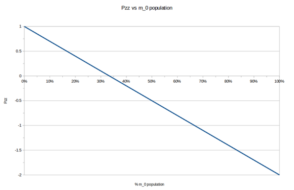
$P_{zz} = (p_1 + p_{-1}) - 2p_0~$.
It has a range of $-2<P_{zz}<1~$.
If the $m_1$ and $m_{-1}$ states are filled, then $(p_1 + p_{-1})=1,~p_0=0$ and $P_{zz}=1~$.
If the combined $m_1$ and $m_{-1}$ states equal the $m_0$ state, then $(p_1+p_{-1})=0.5,~p_0=0.5$ and $P_{zz}=-0.5~$
If the $m_0$ state is filled, then $(p_1 + p_{-1})=0,~p_0=1$ and $P_{zz}=-2~$.
Or, in terms of an overly-simplistic animation,
Deuteron Shape
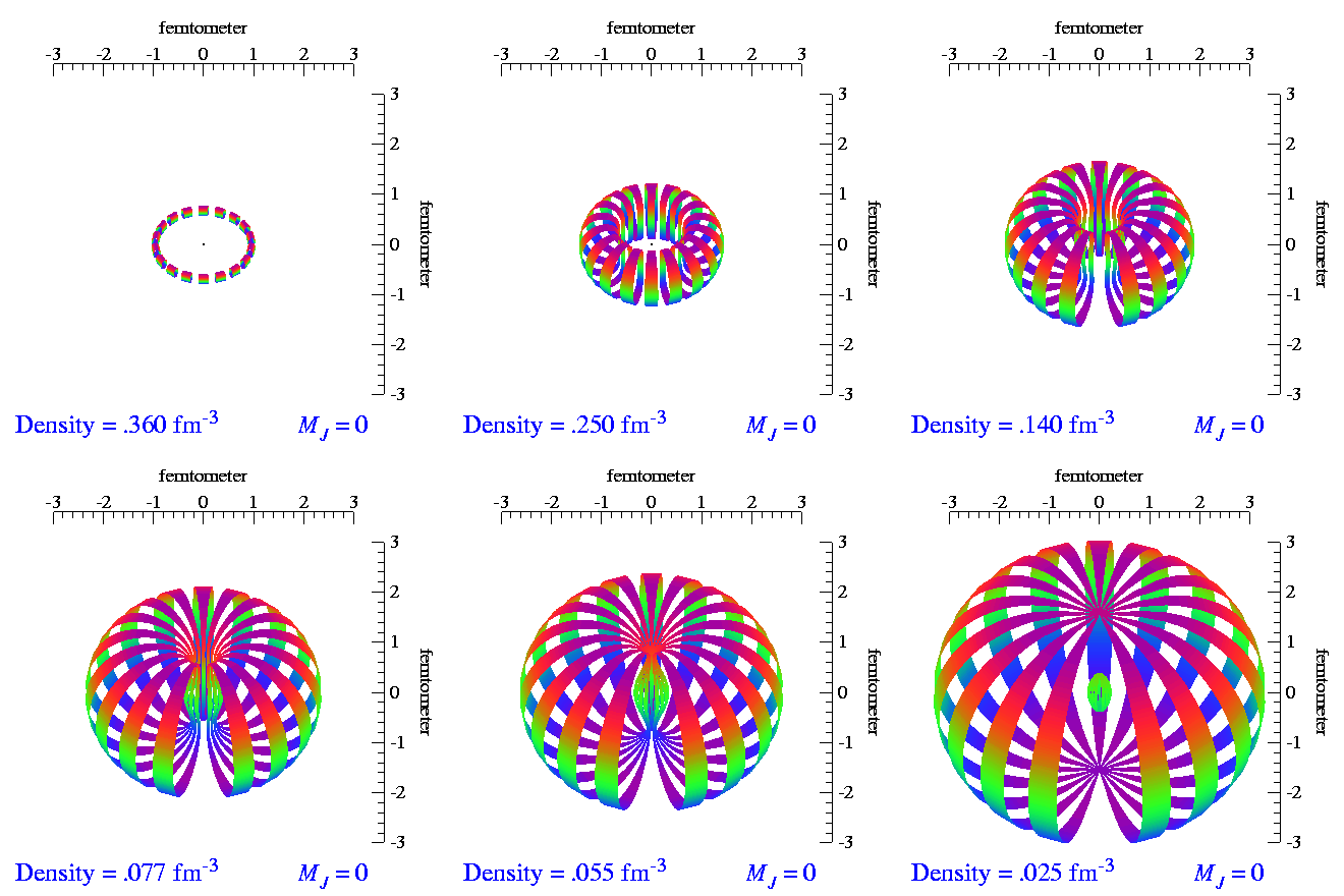
From the video made by S.C. Pieper, et al., I extracted the tensor and vector polarization frames and made repeating videos of each. When we vector-polarize or tensor-polarize, the probability densities for the deuteron look like:
| m_s=±1 | m_s=0 |
|---|---|
 |

|
Tensor Polarization Relation to Vector Polarization
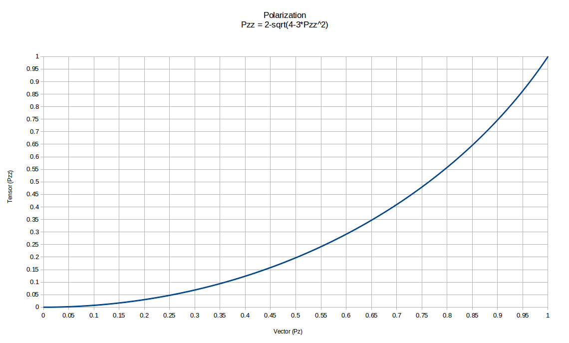
Tensor polarization is related to the vector polarization by $P_{zz}=2-\sqrt{4-3P_{z}^2}$
Deuteron States
From basic quantum mechanics, we know that the possible states for 2 nucleons are
the isospin singlet with S=0:
- $|\uparrow \downarrow> - |\downarrow \uparrow>$ with $m_s=0$, $L=1$
and the isospin triplet with S=1:
- $|\uparrow \uparrow>$ with $m_s=+1$, $L=0$
- $|\uparrow \downarrow> + |\downarrow \uparrow>$ with $m_s=0$, $L=1$
- $|\downarrow \downarrow>$ with $m_s=-1$, $L=2$
For the deuteron, $J=1$ and $P=+1$. This kills both of the $m_s=0$ states, since they cannot simultaneously have $J=1$ and $P=+1$ since $P=(-1)^L$.
This leaves only two possible states:
- $|\uparrow \uparrow>$ with $m_s=+1$, $L=0$
- $|\downarrow \downarrow>$ with $m_s=-1$, $L=2$
Angular Momentum Analysis
Now, let's look at each of these a bit more indepth according to their angular momentum components
| J | $m_J$ | L | $m_L$ | S | $m_S$ | $\pi = -1^L$ | T | $^{2S+1}L_J$ |
|---|---|---|---|---|---|---|---|---|
| 0 | 0 | 0 | 0 | 1 | 0 | + | 1 | $^1 S_0$ |
| 1 | ±1 | 0 | 0 | 1 | ±1 | + | 0 | $^3 S_1$ |
| 1 | 1 | 2 | 1 | 1 | 0 | - | 0 | $^1 P_1$ |
| 1 | 0 | 2 | -1 | 1 | 1 | - | 1 | $^3 P_0$ |
| 1 | 0 | 2 | 1 | 1 | -1 | - | 1 | $^3 P_0$ |
| 1 | 1 | 2 | 1 | 1 | 0 | - | 1 | $^3 P_1$ |
| 1 | 2 | 2 | 1 | 1 | 1 | - | 1 | $^3 P_2$ |
| 1 | 2 | 2 | 2 | 1 | 0 | + | 1 | $^1 D_2$ |
| 1 | 1 | 2 | 2 | 1 | -1 | + | 0 | $^3 D_1$ |
| 1 | -1 | 2 | -2 | 1 | +1 | + | 0 | $^3 D_1$ |
| 3 | 3 | 2 | 2 | 1 | 1 | + | 0 | $^3 D_2$ |
| 3 | 3 | 2 | 2 | 1 | 1 | + | 0 | $^3 D_3$ |
When we remove all of the states that can't exist, we're left with two mentioned in the last section:
| J | $m_J$ | L | $m_L$ | S | $m_S$ | $\pi = -1^L$ | T | $^{2S+1}L_J$ |
|---|---|---|---|---|---|---|---|---|
| 1 | ±1 | 0 | 0 | 1 | ±1 | + | 0 | $^3 S_1$ |
| 1 | 1 | 2 | 2 | 1 | -1 | + | 0 | $^3 D_1$ |
| 1 | -1 | 2 | -2 | 1 | +1 | + | 0 | $^3 D_1$ |
S and D States
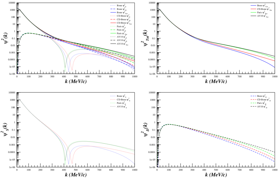
A variety of models have looked at the wavefunction from the S- and D-states.
File:2014-04-24-deuteron-wavefunction-s-d-states.pdf
--E. Long 19:53, 24 April 2014 (UTC)


