Difference between revisions of "Elong-15-05-07"
| (12 intermediate revisions by the same user not shown) | |||
| Line 1: | Line 1: | ||
Going back through the literature, the NIKHEF measurements (for instance [http://journals.aps.org/prl/abstract/10.1103/PhysRevLett.82.3755 the Bouwhuis measurement]) define the polarized D(e,e'd) cross section as | Going back through the literature, the NIKHEF measurements (for instance [http://journals.aps.org/prl/abstract/10.1103/PhysRevLett.82.3755 the Bouwhuis measurement]) define the polarized D(e,e'd) cross section as | ||
| − | + | $$\sigma = \sigma_0\left[ 1 + \frac{A_d^T P_{zz}}{\sqrt{2}} \right]$$ | |
where | where | ||
| − | + | $$ A^T_d = \sum_{i=0}^{2}d_{2i}T_{2i}$$ | |
and | and | ||
| − | + | $$ d_{20} = \frac{3 \cos^2 \theta^* -1}{2},~~d_{21} = -\sqrt{\frac{3}{2}}\sin2\theta^*\cos\phi^*,~~d_{22}=\sqrt{\frac{3}{2}}\sin^2\theta^*\cos 2\phi^*$$ | |
| − | where | + | where $\theta^*$ and $\phi^*$ are in the frame where the $z$ axis is along the $\vec{q}$ (which for us is ~70deg from the beamline) and the $x$ axis is perpendicular to $z$ in the scattering plane. They take the same definitions given by [http://www.sciencedirect.com/science/article/pii/0003491686901739 Donnely and Raskin]: |
[[Image:2015-05-08-coordinate-sys.png|400px]] | [[Image:2015-05-08-coordinate-sys.png|400px]] | ||
| − | If I'm understanding that correctly, then for us | + | If I'm understanding that correctly, then for us $\theta^* = \theta_q = 70^{\circ}$ and $\phi^* = 0^{\circ}$ since our magnetic field will be oriented along the beamline. |
| − | If that's the case, the | + | If that's the case, the $d_{21}\approx -0.787,~~d_{22}\approx 1.08~~$ and $d_{20} \approx -0.3245$. |
| − | Rearranging their top equation to get to what we measure as | + | Rearranging their top equation to get to what we measure as $A_{zz} = \frac{2}{P_{zz}}\left( \frac{\sigma}{\sigma_0} - 1 \right)$, |
| − | + | $A_{zz} = \sqrt{2}\left[ \frac{\sqrt{2}}{P_{zz}}\left( \frac{\sigma}{\sigma_0}-1\right) \right] = \left[ (-0.3245) T_{20} -0.787 T_{21} + 1.08 T_{22}\right] \sqrt{2}$ | |
| − | + | $ A_{zz} = -0.458 T_{20} - 1.113T_{21} + 1.53T_{22}$. | |
The error from this would propagate to | The error from this would propagate to | ||
| − | + | $ \delta T_{20}^{stat} = 2.18\cdot \delta A_{zz}^{stat}$ | |
| − | + | $ \delta T_{20}^{sys} =\sqrt{ \left(2.18\cdot \delta A_{zz}^{sys}\right)^2 + \left(2.42\cdot\delta T_{21}\right)^2 + \left(3.33\cdot\delta T_{22}\right)^2 }$. | |
| − | Looking at the world data for | + | Looking at the world data for $T_{21}$ and $T_{22}$, |
{| border="1" style="text-align:center;" | {| border="1" style="text-align:center;" | ||
| Line 42: | Line 42: | ||
|} | |} | ||
| + | Overlaying the plots on top of each other so they both read in GeV<sup>2</sup> looks like | ||
| − | + | [[Image:2015-05-08-t21-all.png||450px]] [[Image:2015-05-08-t22-all.png||450px]] | |
| − | |||
| − | |||
| − | |||
| − | |||
| − | |||
| − | |||
| − | |||
| − | |||
| − | |||
| − | |||
| − | |||
| − | |||
| − | |||
| − | |||
| − | |||
| − | |||
| + | In discussions with Doug, a reasonable uncertainty on T21 and T22 would be 10%. This was included in the systematics band, along with systematics from Azz, and is shown below. | ||
| − | [[Image:2015-05-07-t20-update.png]] | + | [[Image:2015-05-07-t20-update.png|900px]] |
Latest revision as of 13:43, 18 October 2023
Going back through the literature, the NIKHEF measurements (for instance the Bouwhuis measurement) define the polarized D(e,e'd) cross section as
$$\sigma = \sigma_0\left[ 1 + \frac{A_d^T P_{zz}}{\sqrt{2}} \right]$$
where
$$ A^T_d = \sum_{i=0}^{2}d_{2i}T_{2i}$$
and
$$ d_{20} = \frac{3 \cos^2 \theta^* -1}{2},~~d_{21} = -\sqrt{\frac{3}{2}}\sin2\theta^*\cos\phi^*,~~d_{22}=\sqrt{\frac{3}{2}}\sin^2\theta^*\cos 2\phi^*$$
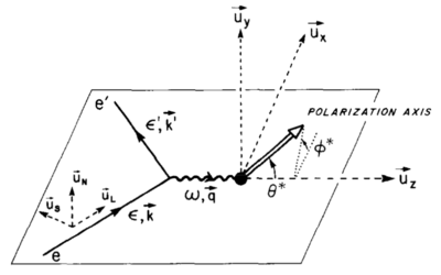
where $\theta^*$ and $\phi^*$ are in the frame where the $z$ axis is along the $\vec{q}$ (which for us is ~70deg from the beamline) and the $x$ axis is perpendicular to $z$ in the scattering plane. They take the same definitions given by Donnely and Raskin:
If I'm understanding that correctly, then for us $\theta^* = \theta_q = 70^{\circ}$ and $\phi^* = 0^{\circ}$ since our magnetic field will be oriented along the beamline.
If that's the case, the $d_{21}\approx -0.787,~~d_{22}\approx 1.08~~$ and $d_{20} \approx -0.3245$.
Rearranging their top equation to get to what we measure as $A_{zz} = \frac{2}{P_{zz}}\left( \frac{\sigma}{\sigma_0} - 1 \right)$,
$A_{zz} = \sqrt{2}\left[ \frac{\sqrt{2}}{P_{zz}}\left( \frac{\sigma}{\sigma_0}-1\right) \right] = \left[ (-0.3245) T_{20} -0.787 T_{21} + 1.08 T_{22}\right] \sqrt{2}$
$ A_{zz} = -0.458 T_{20} - 1.113T_{21} + 1.53T_{22}$.
The error from this would propagate to
$ \delta T_{20}^{stat} = 2.18\cdot \delta A_{zz}^{stat}$
$ \delta T_{20}^{sys} =\sqrt{ \left(2.18\cdot \delta A_{zz}^{sys}\right)^2 + \left(2.42\cdot\delta T_{21}\right)^2 + \left(3.33\cdot\delta T_{22}\right)^2 }$.
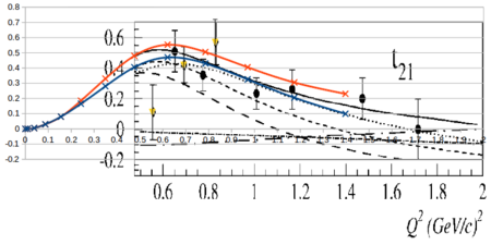
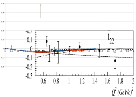
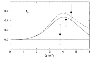
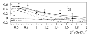
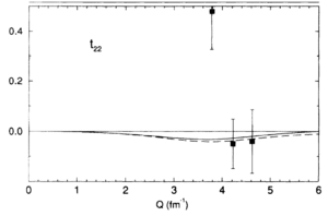
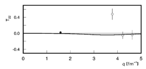
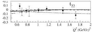
Looking at the world data for $T_{21}$ and $T_{22}$,
| Garcon (1992) | Ferro-Luzzi (1996) | Abbott (2000) |
|---|---|---|
 |
| |
 |
 |
|
Overlaying the plots on top of each other so they both read in GeV2 looks like
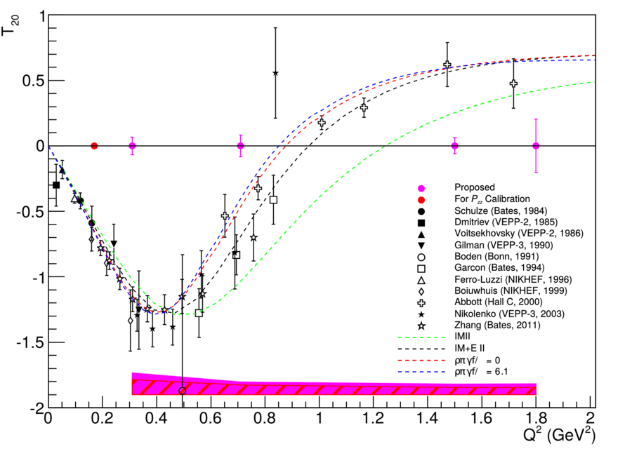
In discussions with Doug, a reasonable uncertainty on T21 and T22 would be 10%. This was included in the systematics band, along with systematics from Azz, and is shown below.
