Difference between revisions of "Elong-14-05-15b"
| Line 147: | Line 147: | ||
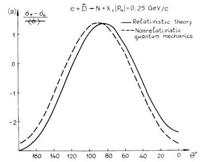
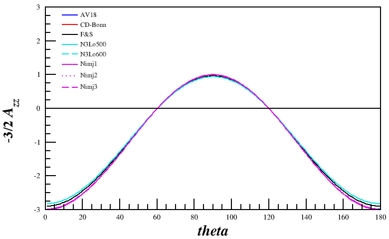
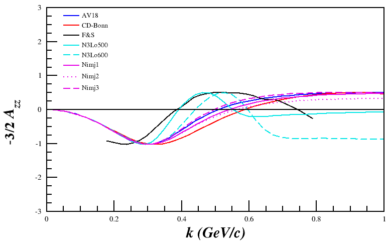
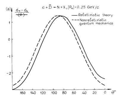
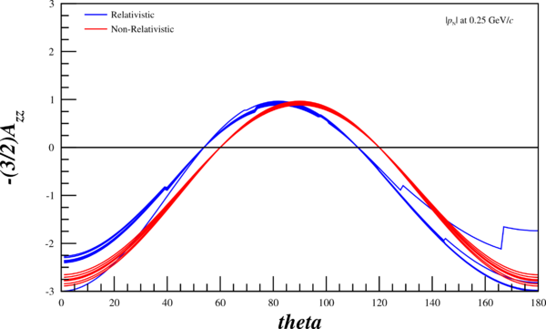
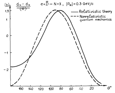
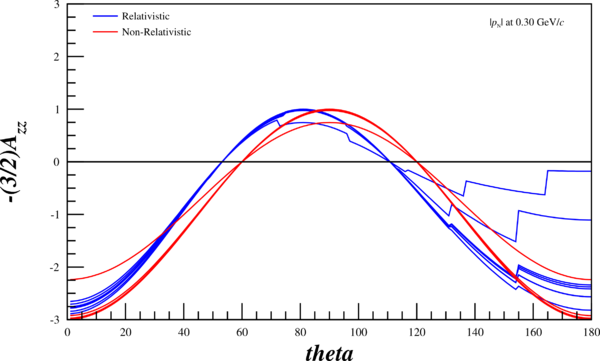
As was mentioned in the relativistic case, there are jagged lines because of the resolution in the tables I have of the wavefunctions. I've added a piece to the script that will find u(k) and w(k) for arbitrary k by taking the tables I already have and creating a linear fit between each of the points on them. When I add this script, I get: | As was mentioned in the relativistic case, there are jagged lines because of the resolution in the tables I have of the wavefunctions. I've added a piece to the script that will find u(k) and w(k) for arbitrary k by taking the tables I already have and creating a linear fit between each of the points on them. When I add this script, I get: | ||
| + | |||
| + | [[Image:2014-05-19-fig-7-6a.png | 400px]] [[Image:2014-05-22-azz-theta-p-025.png | 600px]] | ||
| + | |||
| + | [[Image:2014-05-19-fig-7-6b.png | 400px]] [[Image:2014-05-22-azz-theta-p-030.png | 600px]] | ||
| + | |||
| + | [[Image:2014-05-19-fig-7-6c.png | 400px]] [[Image:2014-05-22-azz-theta-p-035.png | 600px]] | ||
Revision as of 13:13, 22 May 2014
A Note on Azz and Ratios
In the steps mentioned below, following in the footsteps of Frankfurt & Strikman, everything is defined in terms of ratios of the polarized cross-section over the unpolarized cross sections. This leads to
<math>r(0,k) = \frac{\sigma_p^0}{\sigma_u}</math>
<math>r(+1,k) = \frac{\sigma_p^+}{\sigma_u}</math>
<math>r(-1,k) = \frac{\sigma_p^-}{\sigma_u}</math>
To go from these into our Azz observable, which is just the tensor-polarized cross section over the unpolarized cross section, we need <math>\sigma_u = \frac{1}{3}(\sigma_p^0 + \sigma_p^+ + \sigma_p^-)</math> such that
<math>A_{zz} = \frac{\sigma_p^0 - \sigma_u}{\sigma_u} = \frac{\sigma_p^0 - \frac{1}{3}(\sigma_p^0 + \sigma_p^+ + \sigma_p^-)}{\sigma_u}</math>
<math>A_{zz} = \frac{\sigma_p^0}{\sigma_u} - \frac{1}{3}\frac{\sigma_p^0}{\sigma_u} - \frac{1}{3}\frac{\sigma_p^+}{\sigma_u} - \frac{1}{3}\frac{\sigma_p^-}{\sigma_u}</math>
<math>A_{zz} = \frac{2}{3}\frac{\sigma_p^0}{\sigma_u} - \frac{1}{3}\frac{\sigma_p^+}{\sigma_u} - \frac{1}{3}\frac{\sigma_p^-}{\sigma_u}</math>
Now, as we'll see below, <math>r(+1,k)=r(-1,k)=\frac{\sigma_p^+}{\sigma_u}=\frac{\sigma_p^+}{\sigma_u}=\frac{\sigma_p^{\pm}}{\sigma_u}</math>, so
<math>A_{zz} = \frac{2}{3}\frac{\sigma_p^0}{\sigma_u} - \frac{2}{3}\frac{\sigma_p^{\pm}}{\sigma_u}</math>
<math>A_{zz} = \frac{2}{3}\left(\frac{\sigma_p^0}{\sigma_u} - \frac{\sigma_p^{\pm}}{\sigma_u}\right)</math>
So, to go from Frankfurt and Strikman's ratio differences to our measured <math>A_{zz}</math>,
<math>\frac{\sigma_p^0 - \sigma_p^{\pm}}{\sigma_u} = \frac{3}{2}A_{zz}</math>
<math>\frac{\sigma_p^{\pm} - \sigma_p^{0}}{\sigma_u} = -\frac{3}{2}A_{zz}</math>
Non-Relativistic Case
Ratios and Definitions
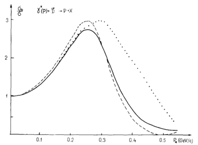
In Frankfurt and Strikman's 1981 report, they go into a bit more detail of how to make the cross section ratios. In particular, on page 258 there is an equation (3.19 and 3.20) for the ratio of cross sections with respect to k,
<math>r(\xi,p)=1+\left(\frac{3(p\xi)^2}{p^2}-1\right)\frac{u(p)w(p)\sqrt{2}+w^2(p)/2}{u^2(p)+w^2(p)}</math>
where <math>\xi</math> is the D-polarization in the D-rest frame, with <math>\xi=(1,\pm i, 0)/\sqrt{2}</math> for <math>\lambda_D=\pm 1</math>, and <math>\xi=(0,0, 1)</math> for <math>\lambda_D=0</math>. Assuming that <math>p\xi=\vec{p}\cdot\xi</math>, this leads to three possible ratios:
<math>r(\pm 1,p)=1+\left(\frac{3p_1^2-3p_2^2}{2\vec{p}\cdot\vec{p}}-1\right)\frac{u(p)w(p)\sqrt{2}+w^2(p)/2}{u^2(p)+w^2(p)}</math>
<math>r(0,p)=1+\left(\frac{3p_3^2}{\vec{p}\cdot\vec{p}}-1\right)\frac{u(p)w(p)\sqrt{2}+w^2(p)/2}{u^2(p)+w^2(p)}</math>.
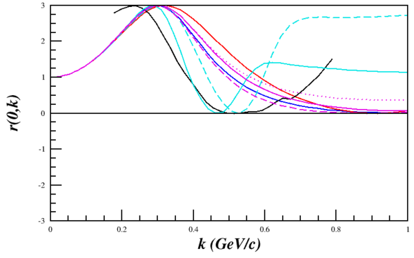
If I am understanding their kinematic variables correctly, then the virtual-photon points along the <math>\hat{z}</math> axis, so in the case of a nucleon being knocked-out at 180deg, <math>p_1=0, p_2=0, p_3=|\vec{p}|</math>. This leads to, in the case of <math>r(0,p)</math> for their Fig. 3.9a,
<math>r(0,p)=1+2\frac{u(p)w(p)\sqrt{2}+w^2(p)/2}{u^2(p)+w^2(p)}</math>,
which can be recreated using the current wavefunctions.
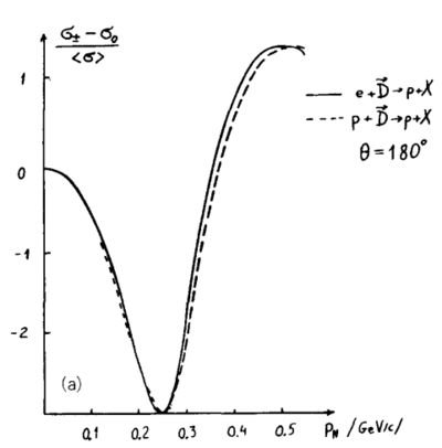
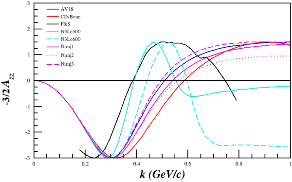
This would make their Fig. 7.5 from their 1988 report simply <math>-\frac{3}{2}A_{zz} = r(\pm 1,p)-r(0,p)</math> for D(e,e'p) with p at 180deg, which can also be reproduced.
Angular Dependence
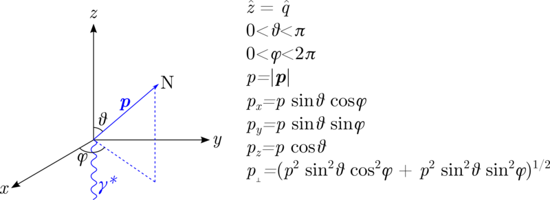
One of the on-going issues I've been having is defining the kinematic directions the same as F&S. Following the convention with <math>z</math> being along the direction of the virtual photon, in the non-relativistic case,
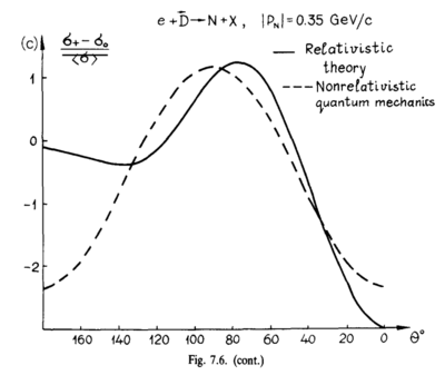
With the light-cone variables being used, I believe that <math>p_1 = p_{\perp} = \sqrt{p_x^2+p_y^2},~~p_2=0,~~p_3=p_z</math>. This lets me recreate their angular distribution in the 1988 report's Fig. 7.6
Note that my assumption for the section above, with the knocked-out proton going at 180deg, as <math>\sin(\pi)=0 \rightarrow p_1=p_2=0, ~\cos(\pi)=1 \rightarrow p_3=p</math> would hold.
Non-relativistic Azz for D(e,e')
In order to find the inclusive D(e,e') Azz, we would simply integrate over all possible angles of the knocked-out nucleon. In the non-relativistic case, this gives
Relativistic Case
Light Cone Definitions
Using Frankfurt and Strikman's 1981 report, we can repeat the process above for the relativistic case,
<math>r(\xi,k)=1+\left(\frac{3(k\xi)^2}{k^2}-1\right)\frac{u(k)w(k)\sqrt{2}+w^2(k)/2}{u^2(k)+w^2(k)}</math>
where <math>\xi</math> is the D-polarization in the D-rest frame, with <math>\xi=(1,\pm i, 0)/\sqrt{2}</math> for <math>\lambda_D=\pm 1</math>, and <math>\xi=(0,0, 1)</math> for <math>\lambda_D=0</math>. Assuming that <math>k\xi=\vec{k}\cdot\xi</math>, this leads to three possible ratios:
<math>r(\pm 1,k)=1+\left(\frac{3k_1^2-3k_2^2}{2\vec{k}\cdot\vec{k}}-1\right)\frac{u(k)w(k)\sqrt{2}+w^2(k)/2}{u^2(k)+w^2(k)}</math>
<math>r(0,k)=1+\left(\frac{3k_3^2}{\vec{k}\cdot\vec{k}}-1\right)\frac{u(k)w(k)\sqrt{2}+w^2(k)/2}{u^2(k)+w^2(k)}</math>.
To do this, we define the following light-cone variables:
<math>\alpha_N = \frac{2(E_p-p_3)}{m_D} = \frac{2(\sqrt{m_N^2+p^2}-p_3)}{m_D}</math>
<math>k_{\perp} = p_{\perp}</math>
<math> k^2 = \frac{m_N^2+p_{\perp}^2}{\alpha_N (2-\alpha_N)} - m_N^2</math>
<math> k_3 = \sqrt{k^2 - k_{\perp}^2}</math>
Angular Dependence
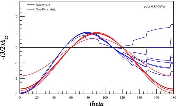
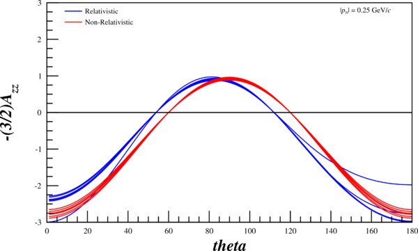
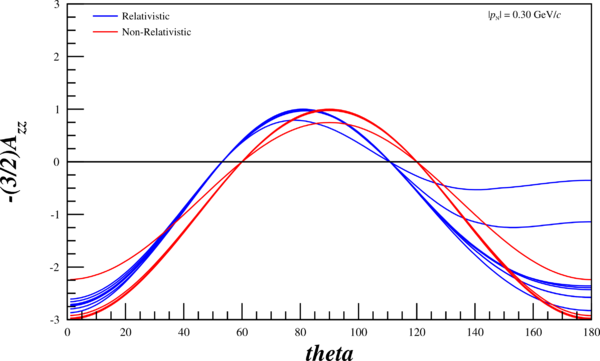
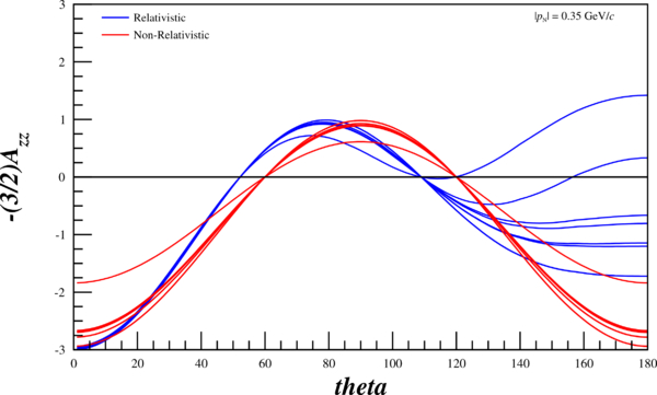
Now, I can re-run my code and attempt to recreate their angular-dependent ratios in the relativistic and non-relativistic case. The multiple lines are the wavefunctions mentioned above, the red curves are the wavefunctions given the non-relativistic treatment, and the blue curves are given the relativistic treatment. Not that the "jaggedness" in the relativistic case comes from having to recalculate <math>r(\pm1,k), ~r(0,k)</math> (as opposed to <math>r(\pm1,p), ~r(0,p)</math>), and that my wavefunction tables don't have the same resolution that I can create through choosing an arbitrary <math>\theta</math>, and thus an arbitrary <math>k</math>
Relativistic D(e,e')
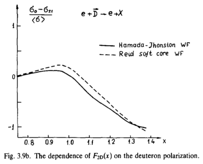
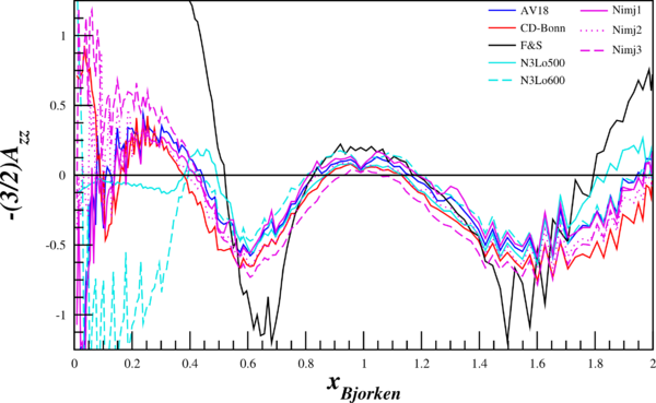
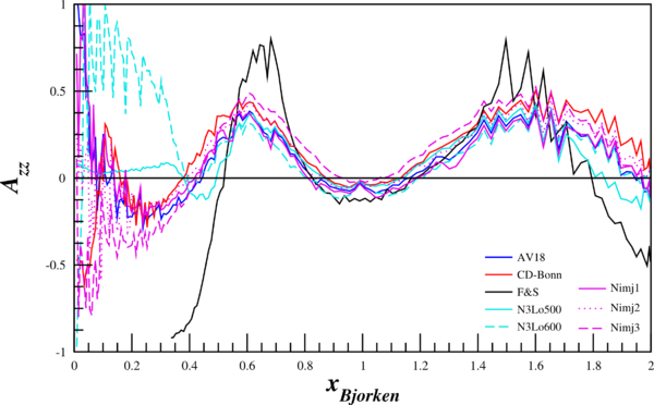
Since the relativistic calculation is working, I calculated an integral of <math>A_{zz}</math> per bin of <math>\alpha</math>, and converted <math>\alpha \rightarrow x</math> and, at <math>Q^2=1.5 \mathrm{GeV}^2</math>, can recreate the Frankfurt and Strikman ratio. It should be noted that, based on the above calculations of <math>\alpha</math>, that it is dependent on <math>p_3</math>, which is dependent on <math>\theta</math>. By taking the integral over <math>\alpha</math>, we are effectively taking an integral over <math>\theta</math>.
To go from <math>\alpha \rightarrow x</math>, I used Eq. 18 from Frankfurt, et al, Phys.Rev. C48 (1993) 2451:
<math>\alpha = 2 - \frac{q_- +2m_N}{2m_N}\left( 1 + \frac{\sqrt{W^2-4m_N^2}}{W}\right)</math>
where
<math>W^2 = 4m_N^2 + 4q_0m_N - Q^2</math>
<math>q_- = q_0 - q_3</math>
<math>q_0 = \frac{Q^2}{2m_Nx}</math>
<math>q_3 = |\mathbf{q}| = \sqrt{Q^2+\frac{Q^4}{4m_N^2x^2}}</math>
I used <math>Q^2=1.5 \mathrm{~GeV}^2</math> and plugged in <math>0\le x\le 2</math>, since the equation fails at <math>x>2</math>. For each point in <math>A_{zz}(\alpha)</math>, I just looked up in the table to convert it to <math>A_{zz}(x)</math>. The results are shown below.
Putting this in terms of our observable <math>A_{zz}</math> looks like the following:
Cleaning Up the Calculations
As was mentioned in the relativistic case, there are jagged lines because of the resolution in the tables I have of the wavefunctions. I've added a piece to the script that will find u(k) and w(k) for arbitrary k by taking the tables I already have and creating a linear fit between each of the points on them. When I add this script, I get:
