Difference between revisions of "Elong-13-05-01"
| Line 17: | Line 17: | ||
This gave <math>f \approx \frac{3\sigma_{D}}{3\sigma_{D}+\sigma{N}} \approx 0.29</math>, as expected. | This gave <math>f \approx \frac{3\sigma_{D}}{3\sigma_{D}+\sigma{N}} \approx 0.29</math>, as expected. | ||
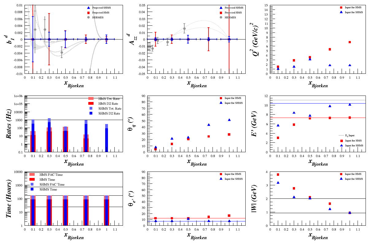
| − | Plugging all this into the rates code gave (NOTE: The error on ''b<sub>1</sub><sup>d</sup>'' is wrong, as discussed below):<br> | + | Plugging all this into the rates code gave ('''NOTE: The error on ''b<sub>1</sub><sup>d</sup>'' is wrong, as discussed below'''):<br> |
[[Image:2013-05-01-fixed-cs.png]] | [[Image:2013-05-01-fixed-cs.png]] | ||
Revision as of 11:46, 1 May 2013
Cross-Section Issue - Fixed
From looking at the dilution factor, f, I found a problem with how the cross-sections were calculated. We know that, naively,
<math>f=\frac{N_{D}}{(N_{D}+N_{N}+N_{He})} = \frac{t\cdot R_{D}}{(t\cdot R_{D}+t\cdot R_{N}+t\cdot R_{He})} = \frac{R_{D}}{(R_{D}+R_{N}+R_{He})} \approx \frac{N_{D}}{N_{D}+N_{N}}\approx \frac{3\sigma_{D}}{3\sigma_{D}+\sigma{N}}\approx \frac{3\cdot 2}{3\cdot 2 + 14}\approx 6/20=0.3</math>.
Originally, I was (wrongly) using
<math>\frac{d^2\sigma^u}{d\Omega dE'} = \left( \frac{d\sigma}{d\Omega} \right) _{\mathrm{Mott}} \left[ \frac{2\cdot \left(\frac{F_1^{X}}{A_X} \right)}{m_{X}}\tan^2\left( \frac{\theta_{e'}}{2} \right) + \frac{\left( \frac{F_2^X}{A_X}\right) }{\nu} \right]</math>
where X = nucleus and <math>\left( \frac{d\sigma}{d\Omega} \right) _{\mathrm{Mott}}=\frac{Z^2 \alpha^2 \hbar^2 c^2}{4E^2\sin^4\left( \frac{\theta}{2} \right)}\cos^2\left( \frac{\theta}{2} \right)</math>.
This gave <math>f \approx 0.062</math>.
The problem came from using a nuclear Mott cross-section but a nucleon structure cross-section. To fix this, I first found the Mott cross-section for a proton,
<math>\left( \frac{d\sigma}{d\Omega} \right) _{\mathrm{Mott}_{\mathrm{p}}}=\frac{1^2 \alpha^2 \hbar^2 c^2}{4E^2\sin^4\left( \frac{\theta}{2} \right)}\cos^2\left( \frac{\theta}{2} \right)</math>,
and then multiplied that by the structure cross-section at the total number of nucleons,
<math>\frac{d^2\sigma^u}{d\Omega dE'} = A_X \left( \frac{d\sigma}{d\Omega} \right) _{\mathrm{Mott}_{\mathrm{p}}} \left[ \frac{2\cdot \left(\frac{F_1^{X}}{A_X} \right)}{m_{X}}\tan^2\left( \frac{\theta_{e'}}{2} \right) + \frac{\left( \frac{F_2^X}{A_X}\right) }{\nu} \right]</math>.
This gave <math>f \approx \frac{3\sigma_{D}}{3\sigma_{D}+\sigma{N}} \approx 0.29</math>, as expected.
Plugging all this into the rates code gave (NOTE: The error on b1d is wrong, as discussed below):

Matching HERMES F1d, dAzzd, and db1d
I wanted to double-check the code against the HERMES data, but this required a few extra steps. First, using the values for <math>A_{zz}^d</math> and <math>b_{1}^d</math> that they measured, along with the formula <math>b_1^d = -\frac{3}{2}A^d_{zz}F^d_1</math>, I found what they were using for <math>F^d_1</math>. The <math>F^d_1</math> they're using is per nucleon, and for HERMES' two highest x points (the rest are inaccessible to the Bosted code because for 0.012<x<0.063, 16.75<W2<42.87, which is outside the W range that the code can handle) they match the code relatively well:
| <x> | Q 2 | HERMES <math>F_1^d</math> | Bosted <math>\frac{F_1^d}{A_d}</math> |
| 0.128 | 2.33 | 1.018 | 0.620 (Outside Bosted "Good" range) |
| 0.248 | 3.11 | 0.496 | 0.486 |
| 0.452 | 4.69 | 0.161 | 0.171 |
This means that the way I was calculating the error <math>\delta b_1^d=\frac{3}{2}\delta A_{zz}^d F_1^d</math> was off by a factor of <math>A_d=2</math>. This was corrected.
I also played a bit with the statistics, trying to match the HERMES results. However, that's a very quick estimate of trying to use the SMHS to copy the HERMES detector, and so the entire like should be taken with a huge grain of salt.
Fixed Rates Code
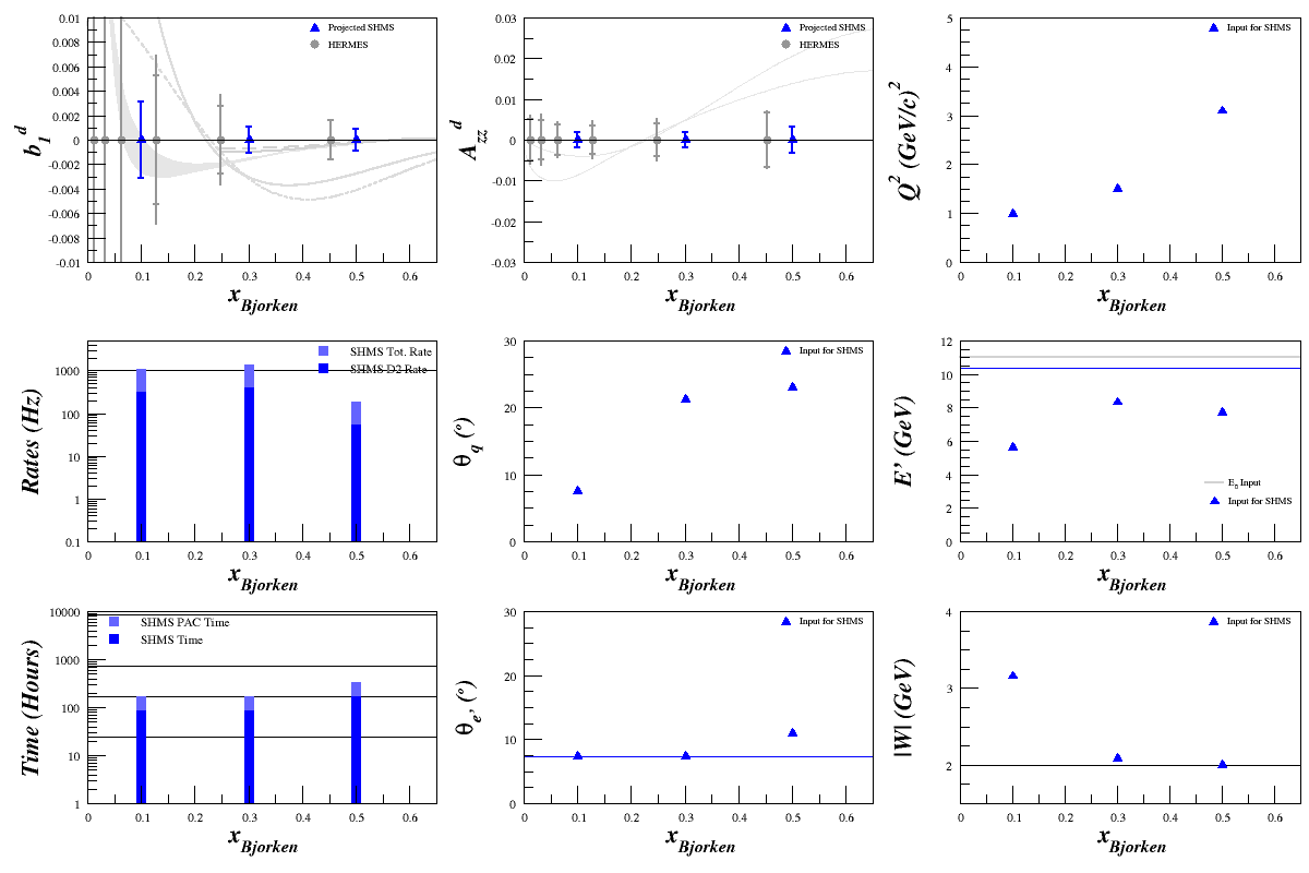
Now that everything is working as it should, I've replotted the lowest three <x> points where we can spend a month taking data. Since the HMS can't get into the range we need for <math>F_1^d</math>, I've removed those calculations. The results (on a re-worked scale to emphasize their value) are:

Where
Target Material ND3 Target Length 3 cm fdil Calculated ~ 0.3 pf 0.65 Pzz 20% E0 11 GeV xBjorken 0.1, 0.3, 0.5 Q2 Variable θq Calculated θe' Calculated E' Calculated W Calculated
Azz Formalism
Just for clarification,
| (1) | <math>R_{\mathrm{Total}} = \mathcal{A}\left[ \mathcal{L}_{\mathrm{He}}\left( \frac{d^2\sigma_{\mathrm{He}}^u}{d\Omega dE'}\right) + \mathcal{L}_{\mathrm{N}}\left( \frac{d^2\sigma_{\mathrm{N}}^u}{d\Omega dE'}\right) + \mathcal{L}_{\mathrm{D}}\left( \frac{d^2\sigma_{\mathrm{D}}}{d\Omega dE'}\right) \right]</math> |
| (2) | <math>R_{\mathrm{Total}} = \mathcal{A}\left[ \mathcal{L}_{\mathrm{He}}\left( \frac{d^2\sigma_{\mathrm{He}}^u}{d\Omega dE'}\right) + \mathcal{L}_{\mathrm{N}}\left( \frac{d^2\sigma_{\mathrm{N}}^u}{d\Omega dE'}\right) + \mathcal{L}_{\mathrm{D}}\left( \frac{d^2\sigma_{\mathrm{D}}^u}{d\Omega dE'}\left[ 1 + \frac{1}{2}P_{zz}A_{zz}^d \right]\right) \right] </math> |
| (2a) | <math>R_{\mathrm{Total}} = \mathcal{A}\left[ \mathcal{L}_{\mathrm{He}} \sigma_{\mathrm{He}}^u + \mathcal{L}_{\mathrm{N}} \sigma_{\mathrm{N}}^u + \mathcal{L}_{\mathrm{D}} \sigma_{\mathrm{D}}^u\left( 1 + \frac{1}{2}P_{zz}A_{zz}^d \right) \right] </math> |
where
| (3) | <math>\mathcal{A} = \left( \Delta\Omega \Delta E' \right)</math> |
| (4) | <math>\mathcal{L}_{\mathrm{He}} = \left[ \mathcal{N}_A \frac{\rho_{\mathrm{He}}}{M_{\mathrm{He}}}\left(1 - p_f\right) \right] \cdot \left( \frac{I_{\mathrm{beam}}}{e} \right) \cdot z_{\mathrm{tgt}}</math> |
| (5) | <math>\mathcal{L}_{\mathrm{N}} = \left[ \mathcal{N}_A \frac{\rho_{\mathrm{ND}_3}}{M_{\mathrm{ND}_3}} p_f \right] \cdot \left( \frac{I_{\mathrm{beam}}}{e} \right) \cdot z_{\mathrm{tgt}}</math> |
| (6) | <math>\mathcal{L}_{\mathrm{D}} = 3\left[ \mathcal{N}_A \frac{\rho_{\mathrm{ND}_3}}{M_{\mathrm{ND}_3}} p_f \right] \cdot \left( \frac{I_{\mathrm{beam}}}{e} \right) \cdot z_{\mathrm{tgt}}</math> |
| (7) | <math>\sigma^u_X = \frac{d^2\sigma^u_X}{d\Omega dE'} = A_X \left( \frac{d\sigma}{d\Omega} \right) _{\mathrm{Mott}_{\mathrm{p}}} \left[ \frac{2\cdot \left(\frac{F_1^{X}}{A_X} \right)}{m_{X}}\tan^2\left( \frac{\theta_{e'}}{2} \right) + \frac{\left( \frac{F_2^X}{A_X}\right) }{\nu} \right]</math> |
| (8) | <math>\left( \frac{d\sigma}{d\Omega} \right) _{\mathrm{Mott}_{\mathrm{p}}}=\frac{1^2 \alpha^2 \hbar^2 c^2}{4E^2\sin^4\left( \frac{\theta}{2} \right)}\cos^2\left( \frac{\theta}{2} \right)</math> |
| (9) | <math>\sigma_D = \frac{d^2\sigma_{\mathrm{D}}}{d\Omega dE'} = \frac{d^2\sigma_{\mathrm{D}}^u}{d\Omega dE'}\left[ 1 + \frac{1}{2}P_{zz}A_{zz}^d \right] </math> |
Then
| (10) | <math>R^+_{\mathrm{Total}} - R^-_{\mathrm{Total}} = \mathcal{A}\left[ \mathcal{L}_{\mathrm{He}} \sigma_{\mathrm{He}}^u + \mathcal{L}_{\mathrm{N}} \sigma_{\mathrm{N}}^u + \mathcal{L}_{\mathrm{D}} \sigma_{\mathrm{D}}^u\left( 1 + \frac{1}{2}P_{zz}^+ A_{zz}^d \right) \right] - \mathcal{A}\left[ \mathcal{L}_{\mathrm{He}} \sigma_{\mathrm{He}}^u + \mathcal{L}_{\mathrm{N}} \sigma_{\mathrm{N}}^u + \mathcal{L}_{\mathrm{D}} \sigma_{\mathrm{D}}^u\left( 1 + \frac{1}{2}P_{zz}^- A_{zz}^d \right) \right] </math> |
| (10a) | <math>R^+_{\mathrm{Total}} - R^-_{\mathrm{Total}} = \mathcal{A}\mathcal{L}_{\mathrm{D}}\sigma_{\mathrm{D}}^u \frac{1}{2}A_{zz} \left[ P_{zz}^+ - P_{zz}^- \right]</math> |
| (11) | <math>R^+_{\mathrm{Total}} + R^-_{\mathrm{Total}} = \mathcal{A}\left[ \mathcal{L}_{\mathrm{He}} \sigma_{\mathrm{He}}^u + \mathcal{L}_{\mathrm{N}} \sigma_{\mathrm{N}}^u + \mathcal{L}_{\mathrm{D}} \sigma_{\mathrm{D}}^u\left( 1 + \frac{1}{2}P_{zz}^+ A_{zz}^d \right) \right] + \mathcal{A}\left[ \mathcal{L}_{\mathrm{He}} \sigma_{\mathrm{He}}^u + \mathcal{L}_{\mathrm{N}} \sigma_{\mathrm{N}}^u + \mathcal{L}_{\mathrm{D}} \sigma_{\mathrm{D}}^u\left( 1 + \frac{1}{2}P_{zz}^- A_{zz}^d \right) \right] </math> |
| (11a) | <math>R^+_{\mathrm{Total}} + R^-_{\mathrm{Total}} = 2\mathcal{A}\left[ \mathcal{L}_{\mathrm{He}} \sigma_{\mathrm{He}}^u + \mathcal{L}_{\mathrm{N}} \sigma_{\mathrm{N}}^u + \mathcal{L}_{\mathrm{D}} \sigma_{\mathrm{D}}^u \right] + \mathcal{A}\mathcal{L}_{\mathrm{D}} \sigma_{\mathrm{D}}^u\left[ \frac{1}{2}P_{zz}^+ A_{zz}^d + \frac{1}{2}P_{zz}^- A_{zz}^d \right] </math> |
If we assume that <math>P_{zz}^+ = -P_{zz}^- = P_{zz}</math>, then
| (12) | <math>R^+_{\mathrm{Total}} - R^-_{\mathrm{Total}} = \mathcal{A}\mathcal{L}_{\mathrm{D}}\sigma_{\mathrm{D}}^u A_{zz} P_{zz}</math> |
| (13) | <math>R^+_{\mathrm{Total}} + R^-_{\mathrm{Total}} = 2\mathcal{A}\left[ \mathcal{L}_{\mathrm{He}} \sigma_{\mathrm{He}}^u + \mathcal{L}_{\mathrm{N}} \sigma_{\mathrm{N}}^u + \mathcal{L}_{\mathrm{D}} \sigma_{\mathrm{D}}^u \right] </math> |
| (14) | <math>A_{\mathrm{meas}} = \frac{R^+_{\mathrm{Total}} - R^-_{\mathrm{Total}}}{R^+_{\mathrm{Total}} + R^-_{\mathrm{Total}}}</math> |
| (14a) | <math>A_{\mathrm{meas}} = \frac{\mathcal{L}_{\mathrm{D}}\sigma_{\mathrm{D}}^u A_{zz} P_{zz}}{2\left[ \mathcal{L}_{\mathrm{He}} \sigma_{\mathrm{He}}^u + \mathcal{L}_{\mathrm{N}} \sigma_{\mathrm{N}}^u + \mathcal{L}_{\mathrm{D}} \sigma_{\mathrm{D}}^u \right]}</math> |
| (14b) | <math>A_{\mathrm{meas}} = \left( \frac{\mathcal{L}_{\mathrm{D}}\sigma_{\mathrm{D}}^u}{\mathcal{L}_{\mathrm{He}} \sigma_{\mathrm{He}}^u + \mathcal{L}_{\mathrm{N}} \sigma_{\mathrm{N}}^u + \mathcal{L}_{\mathrm{D}} \sigma_{\mathrm{D}}^u} \right) \frac{ A_{zz} P_{zz}}{2}</math> |
| (14c) | <math>A_{\mathrm{meas}} = f \frac{ A_{zz} P_{zz}}{2}</math> |
| (15) | <math>A_{zz} = \frac{2 A_{\mathrm{meas}} }{f \cdot P_{zz}}</math> |
In order to get the uncertainty, we'd use
| (16) | <math>\delta A_{zz} = \sqrt{\left( \frac{\partial A_{zz}}{\partial A_{\mathrm{meas}}} \delta A_{\mathrm{meas}} \right)^2 + \left( \frac{\partial A_{zz}}{\partial f} \delta f \right)^2 + \left( \frac{\partial A_{zz}}{\partial P_{zz}} \delta P_{zz} \right)^2 }</math> |
| (16a) | <math>\delta A_{zz} = \sqrt{\left( \delta A_{zz}^{\mathrm{Stat}} \right) ^2 + \left( \delta A_{zz}^{\mathrm{Dil}} \right) ^2 + \left( \delta A_{zz}^{\mathrm{Pol}} \right) ^2 }</math> |
| (16b) | <math>\delta A_{zz} = \sqrt{\left( \delta A_{zz}^{\mathrm{Stat}} \right) ^2 + \left( \delta A_{zz}^{\mathrm{Sys}} \right) ^2 }</math> |
Ignoring <math>\delta A_{zz}^{\mathrm{Sys}}</math> for now (and in all of the plots I'm showing), then
| (17) | <math> \delta A_{zz}^{\mathrm{Stat}} = \frac{\partial A_{zz}}{\partial A_{\mathrm{meas}}} \delta A_{\mathrm{meas}} = \frac{2}{f\cdot P_{zz}} \delta A_{\mathrm{meas}} = \frac{2}{f\cdot P_{zz}}\frac{1}{\sqrt{N_{\mathrm{Total}}}} </math> |
| (17a) | <math> \delta A_{zz}^{\mathrm{Stat}} = \frac{2}{f\cdot P_{zz}\sqrt{t\cdot R_{\mathrm{Total}}}} </math> |
Using the same formalism that HERMES used (which defines <math>F_{1_{\mathrm{HERMES}}}^d = \frac{(1 + Q^2/\nu^2)F_2^d}{2x(1+R)}</math> with <math>F_2^d=\frac{F_2^p + F_2^n}{2}</math> as a per nucleon quantity, which corresponds to the Bosted that uses per nucleus by <math>F_{1_{\mathrm{HERMES}}}^d = \frac{F_{1_{\mathrm{Bosted}}}^d}{A_{\mathrm{D}}} = \frac{F_1^d}{2}</math> -- as described above), we can extract <math>b_1^d</math> and its uncertainty by
| (18) | <math> b_1^d = - \frac{3}{2}A_{zz} \left( \frac{F_1^d}{A_{\mathrm{D}}} \right)= - \frac{3}{2}A_{zz} \left( \frac{F_1^d}{2} \right)</math> |
| (19) | <math> \delta b_1^d =\sqrt{ \left(\frac{\partial b_1^d}{\partial A_{zz}} \delta A_{zz} \right)^2 + \left(\frac{\partial b_1^d}{\partial F_1^d} \delta F_1^d \right)^2 }</math> |
| (19a) | <math> \delta b_1^d =\sqrt{ \left[ - \frac{3}{2} \left( \frac{F_1^d}{2} \right)\delta A_{zz} \right]^2 + \left[ - \frac{3}{2} A_{zz} \left( \frac{1}{2} \right)\delta F_1^d \right]^2 }</math> |
Playing with 30 Days
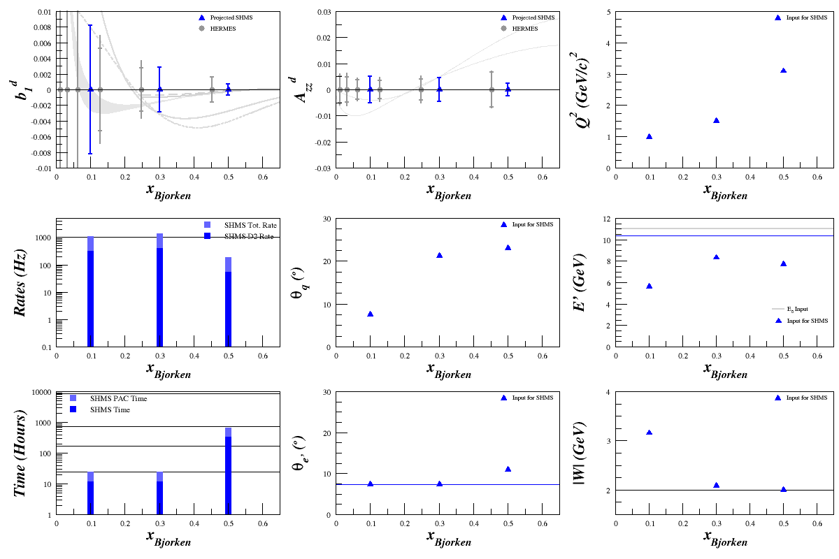
The most interesting point seems to be at <x> ~ 0.5. We can focus the majority of our time there (28 days for <x>=0.5, and 1 day for <x>=0.1 and 0.3), and still get reasonable results for two more points.
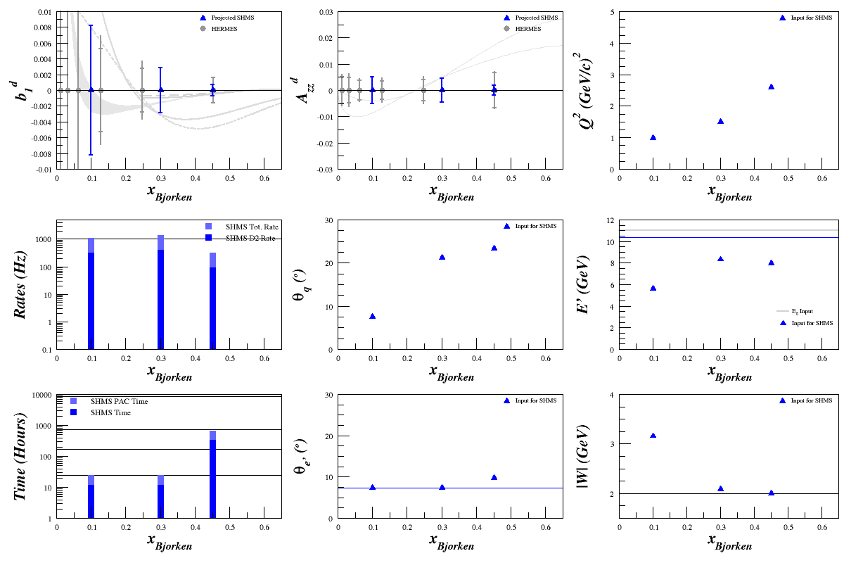
We can do even better if we sit directly on <x> = 0.452 (28 days for <x>=0.452, and 1 day for <x>=0.1 and 0.3), since that lets us pull the angle down a bit and thus get a higher rate:
If we wanted to do better than HERMES for all points, we could do 24 days for <x>=0.5, and 3 days for <x>=0.1 and 0.3
If we wanted to do a lot better than HERMES for all points, we could do 16 days for <x>=0.5, and 7 days for <x>=0.1 and 0.3
If we wanted to split our time up evenly, we could do 10 days for <x>=0.5, 0.3, and 0.1


