Elong-13-09-12

Adding QE Range

Frankfurt and Strikman's 1988 Azz

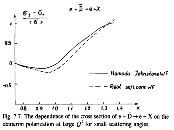
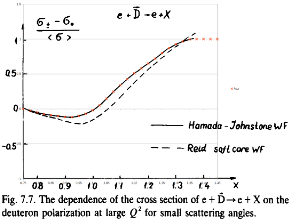
In their 1988 report on Hard Nuclear Processes and Microscopic Structure, Fig. 7.7 plots what appears to be Azz.

I took this plot and super-imposed it onto a plot in a spreadsheet so that I could estimate points along the curve.

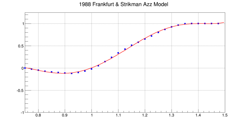
Each of these points, with an uncertainty of ±0.01 on account of my estimating from a previous work without direct points, was then put into a graph in ROOT and fit with a 6th-order polynomial, <math>\sum_{n=0}^6w_n\cdot x^n</math>

<math>n</math>	<math>w_n</math>
0	-5.68296e+01 ± 1.22251e-02
1	2.46102e+02 ± 1.66137e-02
2	-3.51484e+02 ± 1.39410e-02
3	1.11641e+02 ± 1.11237e-02
4	1.63698e+02 ± 8.63783e-03
5	-1.48174e+02 ± 6.15266e-03
6	3.50491e+01 ± 3.63922e-03

This fit was written up as a subroutine for the b1 rates code. It also assumes that at x>1.425, Azz=1 and that at x<0.75, Azz=0. The b1 rates code was then updated to use the previous Kumano curves for x<0.75 and this new QE curve for x>=0.75.

Q2 Scan

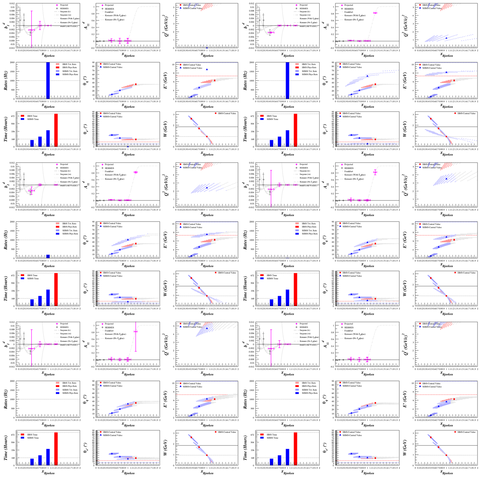
Starting with x=0.5, 0.75, 1.0, and 1.25 and including the Frankfurt and Strikman plot for Azz in the Quasi-Elastic range, I scanned over Q^2 looking for the best rates that fall within the spectrometers' limits.