Elong-15-05-07
Going back through the literature, the NIKHEF measurements (for instance the Bouwhuis measurement) define the polarized D(e,e'd) cross section as
<math>\sigma = \sigma_0\left[ 1 + \frac{A_d^T P_{zz}}{\sqrt{2}} \right]</math>
where
<math> A^T_d = \sum_{i=0}^{2}d_{2i}T_{2i}</math>
and
<math> d_{20} = \frac{3 \cos^2 \theta^* -1}{2},~~d_{21} = -\sqrt{\frac{3}{2}}\sin2\theta^*\cos\phi^*,~~d_{22}=\sqrt{\frac{3}{2}}\sin^2\theta^*\cos 2\phi^*</math>
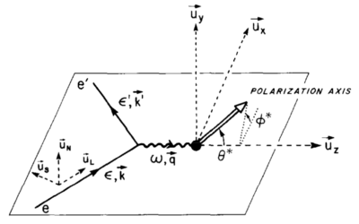
where <math>\theta^*</math> and <math>\phi^*</math> are in the frame where the <math>z</math> axis is along the <math>\vec{q}</math> (which for us is ~70deg from the beamline) and the <math>x</math> axis is perpendicular to <math>z</math> in the scattering plane. They take the same definitions given by Donnely and Raskin:
If I'm understanding that correctly, then for us <math>\theta^* = \theta_q = 70^{\circ}</math> and <math>\phi^* = 0^{\circ}</math> since our magnetic field will be oriented along the beamline.
If that's the case, the <math>d_{21}\approx -0.787,~~d_{22}\approx 1.08~~</math> and <math>d_{20} \approx -0.3245</math>.
Rearranging their top equation to get to what we measure as <math>A_{zz} = \frac{2}{P_{zz}}\left( \frac{\sigma}{\sigma_0} - 1 \right)</math>,
<math>A_{zz} = \sqrt{2}\left[ \frac{\sqrt{2}}{P_{zz}}\left( \frac{\sigma}{\sigma_0}-1\right) \right] = \left[ (-0.3245) T_{20} -0.787 T_{21} + 1.08 T_{22}\right] \sqrt{2}</math>
<math> A_{zz} = -0.458 T_{20} - 1.113T_{21} + 1.53T_{22}</math>.
The error from this would propagate to
<math> \delta T_{20}^{stat} = 2.18\cdot \delta A_{zz}^{stat}</math>
<math> \delta T_{20}^{sys} =\sqrt{ \left(2.18\cdot \delta A_{zz}^{sys}\right)^2 + \left(2.42\cdot\delta T_{21}\right)^2 + \left(3.33\cdot\delta T_{22}\right)^2 }</math>.
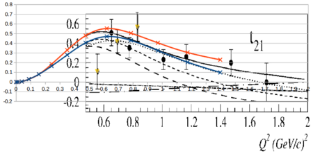
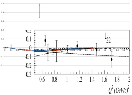
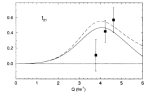
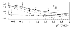
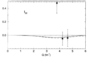
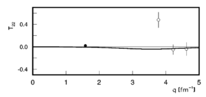
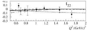
Looking at the world data for <math>T_{21}</math> and <math>T_{22}</math>,
| Garcon (1992) | Ferro-Luzzi (1996) | Abbott (2000) |
|---|---|---|
 |
| |
 |
 |
|
Overlaying the plots on top of each other so they both read in GeV2 looks like
I estimated the following uncertainties for T21 and T22:
| <math>Q^2</math> GeV2 | <math>\delta T_{21}</math> | <math>\delta T_{21}</math> |
|---|---|---|
| 0.2 | 0.99E-02 | 1.92E-02 |
| 0.3 | 4.49E-02 | 2.00E-02 |
| 0.7 | 1.00E-01 | 5.00E-02 |
| 1.5 | 1.00E-01 | 7.19E-02 |
| 1.8 | 1.00E-01 | 8.10E-02 |
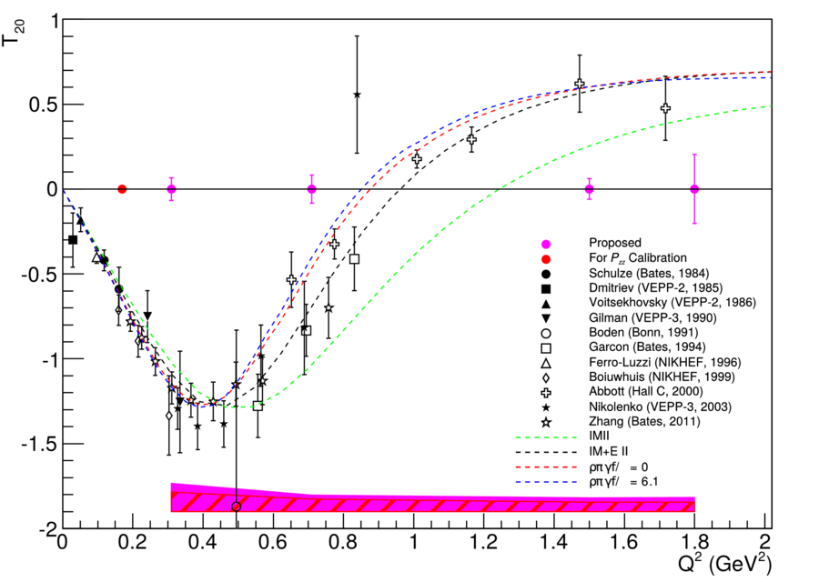
Putting all of this together yields the following plot, where the bars are statistical and band is systematic. Note that the smallest Q^2 point will be a calibration for Azz, and not a measurement of T20 on its own.
