Background Correction for Q²=0.5 data

Overview

In principle, there are two background corrections: a dilution-like correction to account for the extra events, and the asymmetry carried by these extra events. Both will be addressed, individually, in the following.

In addition to the kinematics cuts and other, track based cuts applied to our data, we also have the more fundamental cuts applied to the raw nDet hits. There are two such cuts routinely applied to the data prior to tracking: a cut (window) on the corrected meantime of the individual hits and a cut (minimum) on the energy deposited in the nDet bar by the hit.

The plot below shows a sample spectrum of hit meantimes after the energy cut has been applied. The colored regions correspond to different meantime ranges, all of which have the same width, 10.5ns. The hits that are within the meantime range allowed in our standard tracking process are inside the yellow region; the others are meantime windows of the same width but shifted to either earlier or later. The random hit background apparent in this plot seems to be fairly flat, with only a slight increase towards the coincidence data and a tail thereafter.

Meantime Distribution of Hits. Indicated are the nominal "good" time window, the two early and the late windows. The plot has been edited to shrink the height of the "good" peak. Respective hit counts are indicated, too. Click on picture for a full-size version.

 

Definition of Hit Meantime Windows.

nominal -3.5 ns < tmean < 7.0 ns early 1 -21.5 ns < tmean < -11.0 ns early 2 -32.0 ns < tmean < -21.5 ns late 55.0 ns < tmean < 65.5 ns

Background Rate and Dilution

"Pulse Fiction" credit for this approach goes to Yury G. Kolomensky (as far as I know)

The noise hits constitute the hit background, which is obvisouly also present inside the standard tracking hit meantime window. We could easily subtract the number of noise hits from those observed inside the good time interval but that does not provide us with the background contamination in the tracks, because the distribution throughout the detector is different for noise hits than it is for coincidence hits.

Instead, we need to somehow figure out the impact of the noise hits on the tracking process. An initial approach was to study the tracking done using just the hits from one of the shifted meantime windows. This however introduced the question of how to quantify the effect of mixing: the background hits by themselves and the clean coincidence events by themselves produce different tracks than the sum of the two hit sets. This proved to be a difficult question to resolve.

We therefore switched to another approach: if we can control the relative amount of background inside the standard tracking meantime window we can determine the effect on the resultant tracks. The biggest problem with this approach is that we need to ensure that no bias in introduced. Also, we can only increase the noise level artificially but we cannot reduce it, since that would requires us knowing which events are background -- and then we would not be conducting this exercise.

We make use of the fact that our data acquisition system only allows one hit per trigger (per detector). Thus, any detector element which recorded a hit prior to the coincidence time window was inherrently bared from adding data inside the relevant period. By simply changing the time of these early events we can shift them into the good time interval and make them part of the tracking data set. To ensure no bias is added, we only used events earlier than the coincidence data and so avoid their tail. The idea of this approach comes from a similar method developed for SLAC experiment E154 by Yury G. Kolomensky; we also adopted his term Pulse Fiction for this approach.

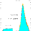
Pulse Fiction. Meantime distribution of hits in the Gen01 neutron detector after hit energy cut and Pulse Fiction hit time shifting. See text for details and explanation.

The plot here shows the hit meantime distribution after the code was patched to change the meantime of hits in the "early 1" window; their times were shifted to the nominal meantime range by adding 18ns to the actual hit meantime. The slight discrepancy in the numbers (< 10,000) between this plot and the one above is entirely due to the difference in rounding in the bin and window definitions in PAW and in FORTRAN.

By comparing the results with those obtained using nomnial reconstruction, we can conclusively determine the impact of adding these hits. Here are two sample plots detailing the results for run 41505, the same one providing the above hit distribution. This overview plot shows the total number of tracks per 0.1ns bin of track time. In blue are the distributions obtained by using either the nominal or the early meantime window seperately, and in yellow the additional tracks created after the early hits have been mapped into the nominal hit meantime window.

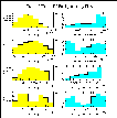
A more detailed plot again compares the track time spectrum for nominal and pulse fiction hit meantimes (left column), and also shows the fractional difference between nominal and pulse fiction tracks (difference divided by nominal). These plots are provided for the entire, uncut track spectrum and for standard proton and neutron definitions. Also indicated in the relative plots is the average fractional difference. Remember that the quoted average is weighed by the number of tracks in the respective time bin; at least that's effectively what happens; the actual calculation is based on the sum of tracks in the allowed track time interval. For the neutrons, we also extrapolated back to find the difference between nominal and clean track spectra and this results in the indicated background level:

Background =

noise data

=

extra - nominal nominal - (extra - nominal)

 

Pulse Fiction Results. See also this plot.
Weighing by the number of nominal STD n tracks, the neutron average becomes 1.99%

Raw Track Counts Fractional Excess (relative) Background Run nominal early pulse fiction all STD p STD n p n 40400 550,055 47,506 584,044 0.0724 0.0355 3.68 % 40479 539,204 46,863 572,538 0.0736 0.0277 1.4 % 2.85 % 40606 522,036 48,650 557,133 0.0796 0.0196 0.1 % 2.00 % 40776 405,491 68,327 454,183 0.1229 0.0220 -0.3 % 2.24 % 40988 813,635 137,597 911,891 0.1241 0.0173 1.76 % 41137 815,110 136,729 912,539 0.1227 0.0197 -0.4 % 2.01 % 41429 791,833 124,649 881,265 0.1170 0.0179 -0.4 % 1.82 % 41505 790,603 130,233 883,865 0.1212 0.0208 -0.4 % 2.12 % simple average 0.0989 0.0207 0.0 % 2.34 % weighed average -0.3 % 1.99 %

 

Proton Background

A definite answer for the negative background in the proton events is not available; there are no indications of an error or a failure in our approach. The most probable answer, therefore, is rooted in the relative rates of events. Due to our specific handling of multi-track events, it is actually possible for an additional hit to decrease the number of coincidence events: if the tracks of the resultant raw event do not allow for simple selection of one of the tracks, all are discarded.

In the case of the neutron events, this highly conservative approach is justified, especially since the number of multi-neutron events is fairly small. For protons, on the other hand, this is not the case. The rate is rather high, and thus also the occurance of multiple tracks. An added noise hit then has a high probability of adversely affecting the overall result, producing a negative background contribution (more hits but fewer tracks). This hypothesis is also supported by the time spectrum of the noise tracks, as is indicated in these summary plots for early time window 1 and time window 2: At times without significant "real" protons, the background contribution is positive (early and late), while during times with high data rates the background contributes negatively.

 

Systematic Limitations, Error Estimation

Several systematic checks were conducted to check the validity of these results. We checked a subset of the runs for dependence on the meantime window providing the additional background data, and we checked for nonlinearity by adding two different background sets into the nominal data set. No problems were found, as is shown in the table below.

To ensure that the results do not depend on the choice of the source meantime window, we repeated the study (with three runs) using the early 2 data, shifted by 28.5ns. Since the background hit rate is very similar, the track rate should increase similarly, providing essentially the same value for the background contamination.

By using both, early 1 and early 2 hits, each mapped as in the individual case, we can increase the background hit level to three times its nominal value. If the track background increases linearly with the hits, the track excess should double and the background level, accounting for the triple rate, should remain the same.

Pulse Fiction Systematic Study.
A plot summarizing the data for each run is linked to from the run's label.

- - - STD N Track Counts - - - Relative Excess (%) Background (%) Run nominal nom + 1 nom + 2 nom + 1 + 2 early 1 early 2 1 & 2 early 1 early 2 1 & 2 40400 563 583 583 601 3.55 3.55 6.75 3.68 3.68 3.49 41137 13775 14047 14062 14313 1.97 2.08 3.91 2.01 2.13 1.99 41505 13101 13373 13367 13617 2.08 2.03 3.94 2.12 2.07 2.01

In interpreting the data above or the plot below, bear in mind that we define the relative excess compared to the standard observed data rate, i.e. a single background contribution. The background, on the other hand, is expressed relative to the clean data, i.e. the uncontaminated rate. As indicated in the caption, the below plot shows an extrapolation of the relative excess to zero background. We could have used the relative background instead, but that quantity is determined by linearly extrapolating the difference between the nominal event rate and the pulse fiction set under consideration. The fit is somewhat more general.

Excess Extrapolation for Error Estimate. This plot shows the results of fitting the systematic data. Each run's data and fit are plotted in a different color. The blue and purple data sets, as well as the overall fit, overlap completely. The indicated fit results are for the overall fit. Only counting statistics are considered in the fitting process. Horizontal offsets are for visualization only.

The offset value is not the actually interesting quantity here, however. We have a more significant value for the average background from the large sample average above. This systematic subset is only intended to quantify the extrapolation error. Since we are looking at relative background rates, the error of the offset here is to be interpreted as the absolute error of the relative background. Specifically, using the above overall result, this means that our neutron data have (1.99 +/- 0.076) % background. This means the systematic error from the background rate correction is less than 0.1% relative. We could also consider using the spread in the individual runs' results as an error estimate -- or even two independent factors that contribute to the total error. The result would still be merkedly less than 1%, though...

 

Kinematic Bins

The above results are highly sensitive to the number of STD n events in the run; some are therefore only marginally meaningful. We could simply average the results and come up with a safe 2% background contamination, but the earlier runs, which have a larger value, are at different kinematics and might actually have a higher background rate...

Since we split the data into kinematic bins prior to drawing any physics conclusions, we also consider the background in each of these bins seperately. Since the same statistical limitations are present here, even more so, only average quantities are really useful. The values given in the following tables have therefore been averaged, with the number of STD neutron events as weight. The detailed values (in a dense form) are available here, a sample plot of the details is available for run 41505, and the averaged data are plotted here. For the background values indicated here, in percent, the asymmetry correction is thus applied as <corrected asymmetry>   =   <raw asymmetry>   *   (1 + <background in % >/100)

 

Average Background in Kinematic Bins. A plot is available here. The values shown are the background rate, in percent, relative to the clean data, i.e. without background. The data are thus 100% in each bin.

bin Center Background 1 2.0113 1.3 % 2 2.0298 1.5 % 3 2.0483 1.8 % 4 2.0668 1.9 % 5 2.0853 2.0 % 6 2.1038 3.3 % 7 2.1223 5.5 % 8 2.1408 11.7 % Eprime Bins

bin Center Background 1 -35 2.6 % 2 -25 2.5 % 3 -15 1.3 % 4   -5 1.6 % 5     5 1.9 % 6   15 2.1 % 7   25 2.2 % 8   35 2.5 % ypos Bins

bin Center Background 1 0.0069 -0.3 % 2 0.0206   0.7 % 3 0.0344   1.3 % 4 0.0481   1.5 % 5 0.0619   1.7 % 6 0.0756   2.7 % 7 0.0894   2.9 % 8 0.1031   3.8 % theta_pq Bins

bin Center Background 1 166 2.2 % 2 170 2.2 % 3 174 1.4 % 4 178 0.7 % 5 182 0.8 % 6 186 1.7 % 7 190 3.3 % 8 194 3.4 % theta_np Bins

Background Asymmetry Correction

The background asymmetry, however, is a different story. Here, we do not actually care about the exact time of the (background) tracks, as long as both beam helicities are treated equally. If we are then looking at a time where the hits that might have entered into the creation of the track are guaranteed to be background hits, the resulting track asymmetry is bound to be representative of the background.

The results are tabulated below and plotted here. The values are based on tracks from the early and late time windows, as defined previously. The time ranges are also indicated in the plot of the track time spectrum below. These data are asymmetries corrected for beam and target polarization, as well as BCA. They are thus comparable to similarly corrected data asymmetries but no dilution factor has been applied.

Time Distribution of Tracks. Indicated are the tracks falling inside the early, nominal and late time windows. Initially, for this study, reconstruction was done using all> hits, after energy cut; more recently, the hit meantime window was set to -40ns<mt<80ns, large enough to eliminate any edge effects.

To apply an asymmetry correction to the data, we simply subtract the background asymmetry from the data asymmetry, weighing them by their respective statistical error bar. Note that the resulting statistical error is not obtained by adding the the weights but by subtracting the error's weight, such as to increase the resulting error. To put it into math:

A = ( A1/o12 - A2/o22 ) / ( 1/o12 - 1/o22 )

oA = 1/sqrt( 1/o12 - 1/o22 )

Here we use A₁ for the contaminated asymmetry, A₂ for the background's asymmetry, A for the corrected asymmetry and o₁,o₂,o_A for the respective errors. The reason for this is that we do not want to improve the statistics due to the removal of the background, which would result from the standard equation. Note that this only works if the correction being removed has a bigger error (less statistics) than the raw quantity being corrected.

If we take the stick 2 average of the early time window to be the proper background asymmetry value, -0.0744 +/- 0.0786, then a simple statistics-weighed average changes the stick 2 asymmetry from 0.05145 +/- 0.00352 (incl. 0.71769 dilution factor) to 0.05161 +/- 0.00352 (based on butcher v16 data). However, we have established that the background contamination of the neutron data has 0 asymmetry within errors, and we are correcting for the dilution from these events explicitly. This means we already have fully accounted for the background and this calculation would constitute a double-counting of the background.

Background Asymmetry Results. A summary plot can be found here. These data are asymmetries corrected for beam and target polarization, as well as BCA. They are thus comparable to similarly corrected data asymmetries, but note that no dilution factor has been applied!

- - - neutron - - - - - - proton - - - Run No. (runs) before after before after 40400 1.1525 +/- 0.5468 0.9057 +/- 0.6155 0.0371 +/- 0.4072 -0.2419 +/- 0.4740 40479 0.2493 +/- 0.4459 0.2049 +/- 0.4324 -0.2763 +/- 0.3212 0.2975 +/- 0.3442 40606 1.2524 +/- 0.7493 -0.2140 +/- 0.8706 -0.2497 +/- 0.5753 1.2170 +/- 0.6169 40776 1.0914 +/- 0.7403 0.2165 +/- 0.9248 -0.4107 +/- 0.6264 0.8351 +/- 0.7191 40853 -0.1503 +/- 0.2726 -0.1708 +/- 0.3101 -0.2714 +/- 0.2297 0.0049 +/- 0.2600 40920 -0.1120 +/- 0.3330 0.4488 +/- 0.4057 0.1229 +/- 0.2696 0.0620 +/- 0.3091 40988 0.1688 +/- 0.3574 0.7703 +/- 0.4222 0.2298 +/- 0.2857 -0.5704 +/- 0.3331 41137 -0.4399 +/- 0.3655 -0.7112 +/- 0.4538 0.1437 +/- 0.3223 -0.2000 +/- 0.3677 41163 -0.2206 +/- 0.2389 0.0242 +/- 0.2932 -0.2515 +/- 0.1963 0.4738 +/- 0.2254 41211 -0.1014 +/- 0.2528 -0.0764 +/- 0.2932 0.1311 +/- 0.2030 -0.3031 +/- 0.2358 41290 -0.1031 +/- 0.2262 0.0545 +/- 0.2697 -0.0755 +/- 0.1837 -0.0927 +/- 0.2166 41359 0.1434 +/- 0.2309 0.4285 +/- 0.2730 0.3291 +/- 0.1942 -0.3041 +/- 0.2170 41429 0.1937 +/- 0.3078 -0.0102 +/- 0.3552 -0.2181 +/- 0.2540 0.1320 +/- 0.2834 41505 -0.0637 +/- 0.2649 0.1761 +/- 0.3093 0.6557 +/- 0.2199 -0.2797 +/- 0.2548 41552 -0.4686 +/- 0.3012 -0.1650 +/- 0.3645 -0.1447 +/- 0.2450 -0.8715 +/- 0.2642 41602 0.1058 +/- 0.2442 -0.3830 +/- 0.2988 0.0647 +/- 0.2010 0.0194 +/- 0.2333 all (16) -0.0155 +/- 0.0759 0.0592 +/- 0.0895 0.0347 +/- 0.0620 -0.0951 +/- 0.0707 stick1 (4) 0.7788 +/- 0.2889 0.3300 +/- 0.3090 -0.1998 +/- 0.2167 0.3580 +/- 0.2394 stick2 (12) -0.0744 +/- 0.0786 0.0344 +/- 0.0935 0.0556 +/- 0.0648 -0.1384 +/- 0.0740 s2 top (7) -0.0640 +/- 0.1095 0.0890 +/- 0.1289 0.1293 +/- 0.0912 -0.2976 +/- 0.1028 s2 bot (5) -0.0854 +/- 0.1129 -0.0262 +/- 0.1357 -0.0193 +/- 0.0919 0.0331 +/- 0.1067 top+ (3) -0.1040 +/- 0.1521 0.0871 +/- 0.1786 0.0189 +/- 0.1269 -0.3748 +/- 0.1409 top- (5) 0.0093 +/- 0.1488 0.1089 +/- 0.1710 0.1726 +/- 0.1215 -0.1285 +/- 0.1377 bot+ (4) -0.0337 +/- 0.1341 -0.0934 +/- 0.1624 -0.0950 +/- 0.1096 0.1759 +/- 0.1270 bot- (4) 0.1089 +/- 0.1831 0.2082 +/- 0.2156 0.0869 +/- 0.1465 -0.1224 +/- 0.1694 s1 + (1) 1.2524 +/- 0.7493 -0.2140 +/- 0.8706 -0.2497 +/- 0.5753 1.2170 +/- 0.6169 s1 - (3) 0.6961 +/- 0.3131 0.4084 +/- 0.3305 -0.1916 +/- 0.2339 0.2057 +/- 0.2597 s2 + (6) -0.0886 +/- 0.1015 -0.0078 +/- 0.1213 -0.0420 +/- 0.0838 -0.1017 +/- 0.0955 s2 - (6) -0.0530 +/- 0.1242 0.0959 +/- 0.1466 0.2003 +/- 0.1020 -0.1937 +/- 0.1173 s2+top (3) -0.1040 +/- 0.1521 0.0871 +/- 0.1786 0.0189 +/- 0.1269 -0.3748 +/- 0.1409 s2+bot (3) -0.0763 +/- 0.1363 -0.0891 +/- 0.1653 -0.0892 +/- 0.1116 0.1298 +/- 0.1298 s2-top (4) -0.0208 +/- 0.1579 0.0911 +/- 0.1862 0.2476 +/- 0.1312 -0.2097 +/- 0.1503 s2-bot (2) -0.1053 +/- 0.2013 0.1038 +/- 0.2376 0.1281 +/- 0.1622 -0.1688 +/- 0.1874