Elong-13-04-29

Rates Update

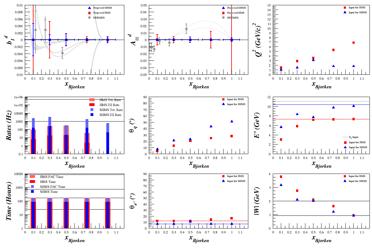
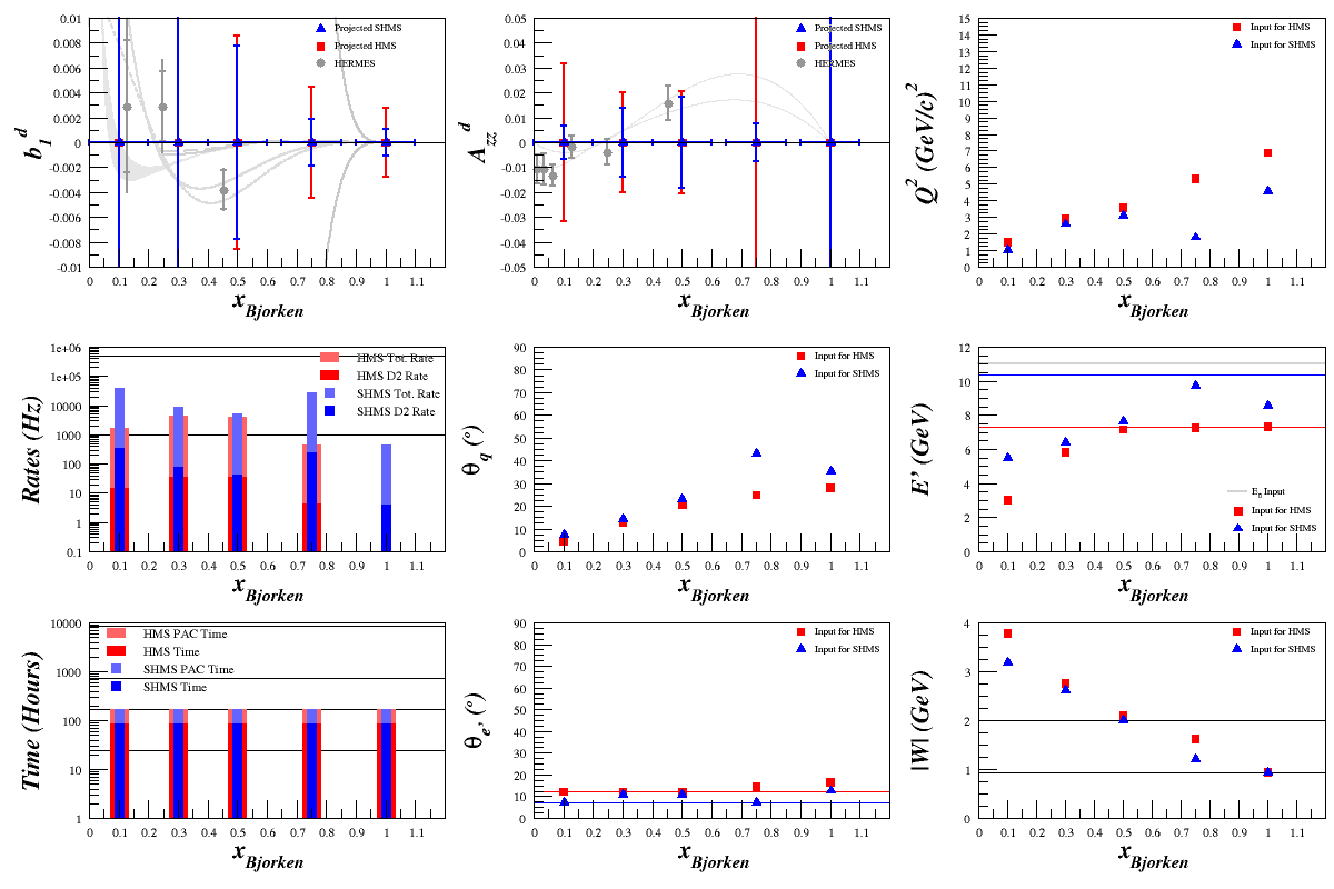
→ For the plots below, I assume the following:

Target Material	ND3
Target Length	3 cm
fdil	(See below)
pf	0.65
Pzz	20%
E0	11 GeV
xBjorken	0.1, 0.3, 0.5, 0.75, 1.0
Q2	Variable
θq	Calculated
θe'	Calculated
E'	Calculated
W	Calculated

→ θ_e' and E' limits were added for each spectrometer

→ Error bars shown are statistical only

→ F1 and F2 are calculated using the Bosted fits, which lets us extend into a higher <x> range

→ It is valid for 0<W<3.2 GeV and 0.2<Q²<5 GeV²

→ The error bars are calculated from:

$dA_{zz} = \left( \frac{4}{f_{\mathrm{dil}}N_DP_{zz}} \right) \cdot \left( \frac{1}{\sqrt{t\cdot R_D}} \right)$

$db_1^d = |1.5\cdot dA_{zz}| \cdot F_1^d$

Dilution Factor

I've been a bit confused by the dilution factor, f. It stems from:
$f=\frac{N_{D}}{(N_{D}+N_{N}+N_{He})} = \frac{t\cdot R_{D}}{(t\cdot R_{D}+t\cdot R_{N}+t\cdot R_{He})} = \frac{R_{D}}{(R_{D}+R_{N}+R_{He})} \approx \frac{N_{D}}{N_{D}+N_{N}}\approx \frac{3\sigma_{D}}{3\sigma_{D}+\sigma{N}}\approx \frac{3\cdot 2}{3\cdot 2 + 14}\approx 6/20=0.3$, but I'm having difficulties matching that and the trouble seems to be coming from the cross-sections.

The cross section I'm using is

$\frac{d^2\sigma^u}{d\Omega dE'} = \left( \frac{d\sigma}{d\Omega} \right) _{\mathrm{Mott}} \left[ \frac{2\cdot F_1^{X}}{m_{X}}\tan^2\left( \frac{\theta_{e'}}{2} \right) + \frac{F_2^X}{\nu} \right]$

where X = nucleus and $\left( \frac{d\sigma}{d\Omega} \right) _{\mathrm{Mott}}=\frac{Z^2 A^2 \hbar^2 c^2}{4E^2\sin^4\left( \frac{\theta}{2} \right)}\cos^2\left( \frac{\theta}{2} \right)$.

Using the Bosted code, I get

	<x>	Q 2	$F_1^X$	$F_2^X$	$\frac{d^2\sigma^u_X}{d\Omega dE'}$
D	0.1	1.01	2.16	0.558	$1.57 \cdot 10^{-7}$
N	0.1	1.01	14.8	3.99	$9.40 \cdot 10^{-5}$
D	0.3	1.50	0.816	0.509	$2.35 \cdot 10^{-7}$
N	0.3	1.50	5.72	3.73	$1.75 \cdot 10^{-4}$
D	0.5	3.10	0.284	0.258	$2.12 \cdot 10^{-8}$
N	0.5	3.10	1.95	1.79	$1.35 \cdot 10^{-5}$
D	0.75	1.75	0.162	0.129	$1.35 \cdot 10^{-7}$
N	0.75	1.75	0.765	0.632	$6.40 \cdot 10^{-5}$
D	0.98	1.80	0.197	0.157	$2.08 \cdot 10^{-7}$
N	0.98	1.80	0.190	0.322	$4.13 \cdot 10^{-5}$

This, however, gives $f\approx 0.005$.

If, instead, I use $\frac{d^2\sigma^u}{d\Omega dE'} = \left( \frac{d\sigma}{d\Omega} \right) _{\mathrm{Mott}} \left( \frac{2F_1^X}{m_Xc^2} \right) \left[ \tan^2\left(\frac{\theta}{2}\right) +\frac{Q^2}{2\nu^2} \right]$, then I get

	<x>	Q 2	$F_1^X$	$F_2^X$	$\frac{d^2\sigma^u_X}{d\Omega dE'}$
D	0.1	1.01	2.16	0.558	$1.27 \cdot 10^{-7}$
N	0.1	1.01	14.8	5.70	$9.40 \cdot 10^{-6}$
D	0.3	1.50	0.816	0.509	$2.44 \cdot 10^{-7}$
N	0.3	1.50	5.72	1.12	$1.75 \cdot 10^{-5}$
D	0.5	3.10	0.284	0.258	$2.32 \cdot 10^{-8}$
N	0.5	3.10	1.95	1.05	$1.35 \cdot 10^{-6}$
D	0.75	1.75	0.162	0.129	$2.53 \cdot 10^{-7}$
N	0.75	1.75	0.765	7.84	$6.40 \cdot 10^{-6}$
D	0.98	1.80	0.197	0.157	$5.08 \cdot 10^{-7}$
N	0.98	1.80	0.190	0.322	$3.21 \cdot 10^{-6}$

with $f \approx 0.062$ for <x>=0.1, 0.3, and 0.5, $f \approx 0.088$ for <x>=0.75, and $f \approx 0.32$ for <x>=0.98.

The above are for specific cross-checks. If I take input the second method into the code, which scans cross-sections only within the range that the SMHS can accept, and finding $f = \frac{R_D}{R_D + R_N + R_{He}}$ then we get $f \approx 0.065 - 0.080$ and the following statistics:

Maximizing Rate (Minimizing dA_zz)

Using $\frac{d^2\sigma^u}{d\Omega dE'} = \left( \frac{d\sigma}{d\Omega} \right) _{\mathrm{Mott}} \left[ \frac{2\cdot F_1^{X}}{m_{p}}\tan^2\left( \frac{\theta_{e'}}{2} \right) + \frac{F_2^X}{\nu} \right]$

If we set the spectrometer such that we aim to increase the rate as high as we can, it will get us the lowest (statistically) achievable A_zz.

The settings above give us the highest rates we can achieve, and thus the lowest error bars on A_zz. Each of the <x> values is set over the course of 1 PAC-week, allowing us to take any four of the above points.

<x>	dAzz with SHMS	dAzz with HMS	db1 with SHMS	db1 with HMS
0.1	0.00619	0.0316	0.0200	0.0770
0.3	0.00564	0.0203	0.00691	0.0244
0.5	0.0192	0.0204	0.00819	0.00853
0.75	0.00765	0.0593	0.00187	0.00444
1.0	0.0136	0.699	0.00421	0.00279

The db1 Problem

→ Since db₁ is calculated from $db_1^d = |1.5\cdot dA_{zz}| \cdot F_1^d$, it is dependent upon F₁
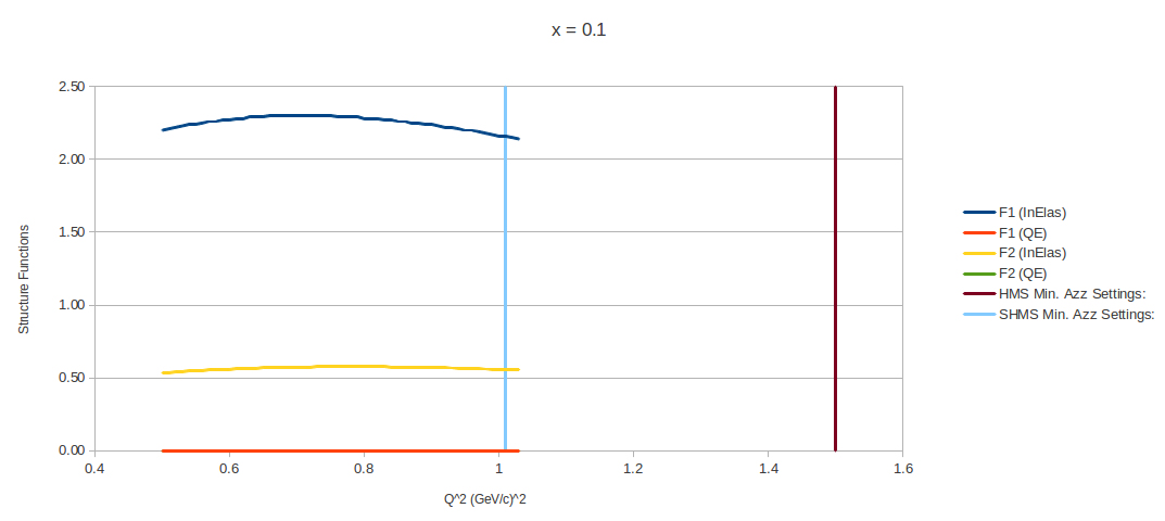
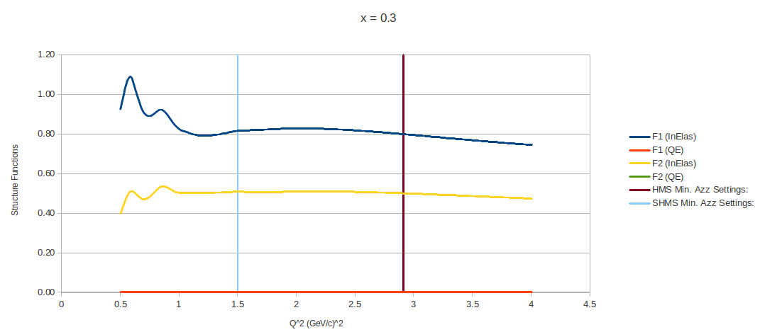
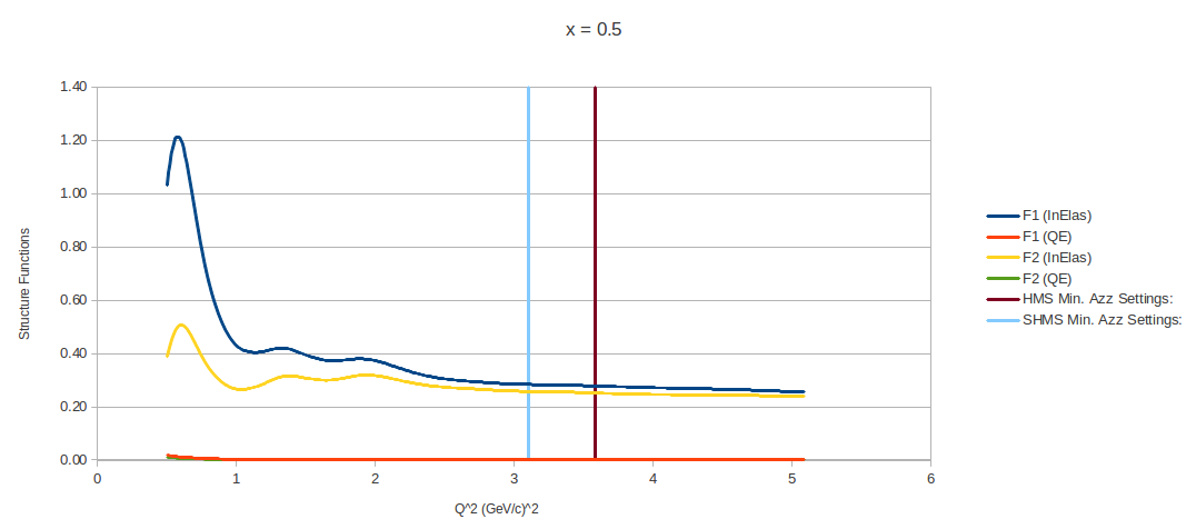
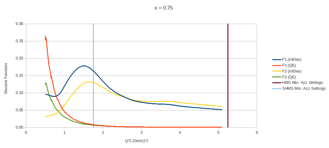
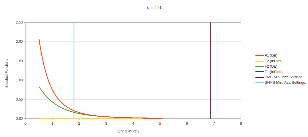
→ For each of the <x> values that I've been looking at, the following show what the Bosted code produces as a function of Structure Function vs. Q^2
→ For the plots below, the structure functions are calculated within the allowable Q ² and W² ranges of the Bosted fits
→ The two vertical lines indicate the Q ² values where dA_zz has been minimized

Structure Function vs. Q ² for <x>=0.1

Structure Function vs. Q ² for <x>=0.3

Structure Function vs. Q ² for <x>=0.5

Structure Function vs. Q ² for <x>=0.75

Structure Function vs. Q ² for <x>=1.0

Minimizing db₁

Using $\frac{d^2\sigma^u}{d\Omega dE'} = \left( \frac{d\sigma}{d\Omega} \right) _{\mathrm{Mott}} \left[ \frac{2\cdot F_1^{X}}{m_{p}}\tan^2\left( \frac{\theta_{e'}}{2} \right) + \frac{F_2^X}{\nu} \right]$

If we set the spectrometer at the lowest allowed values of F1 (from above), it will get us the lowest (statistically) achievable db₁.

The settings above give us the lowest statistical error bars we can achieve on db₁. Each of the <x> values is set over the course of 1 PAC-week, allowing us to take any four of the above points.

<x>	dAzz with SHMS	dAzz with HMS	db1 with SHMS	db1 with HMS
0.1	0.00656	0.0316	0.0211	0.0770
0.3	0.0140	0.0203	0.0171	0.0244
0.5	0.0183	0.0204	0.00779	0.00853
0.75	0.00765	0.0593	0.00187	0.00444
1.0	0.0596	0.699	0.00103	0.00279

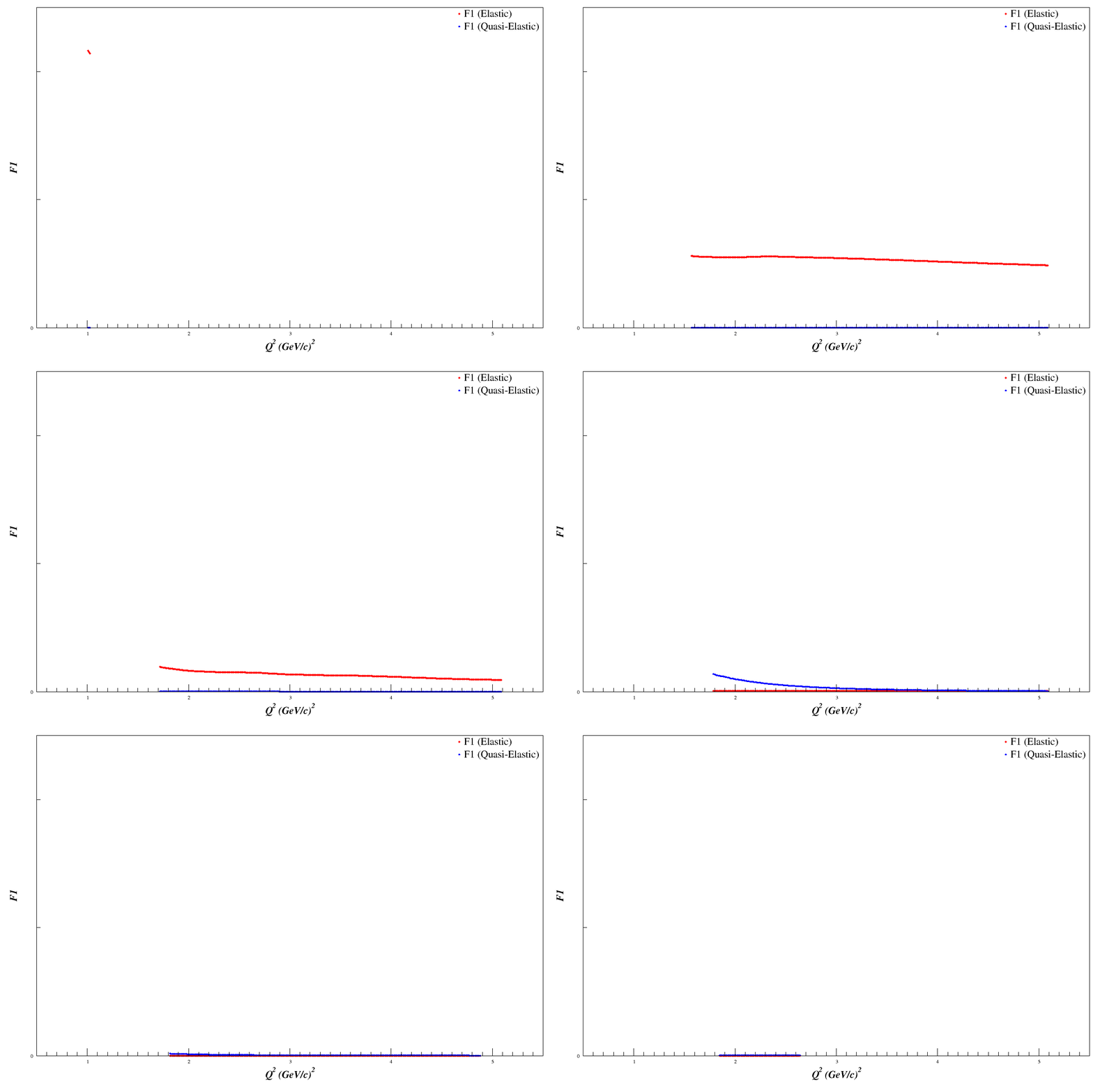
F1 Scan

Using the Bosted fits and scanning over the <x> range 0.1<x<1.5, in increments of 0.001, we can see that F1 will drop as we go to higher Q ². This should cause the error bars on b^d₁ to drop accordingly, since $db_1^d = |1.5\cdot dA_{zz}| \cdot F_1^d$

This plot shows the Bosted F1 curves over a range in <x>, using kinematics that we can reach. Individual frames can be found here.

Summary

Using $\frac{d^2\sigma^u}{d\Omega dE'} = \left( \frac{d\sigma}{d\Omega} \right) _{\mathrm{Mott}} \left( \frac{2F_1^X}{m_Xc^2} \right) \left[ \tan^2\left(\frac{\theta}{2}\right) +\frac{Q^2}{2\nu^2} \right]$,

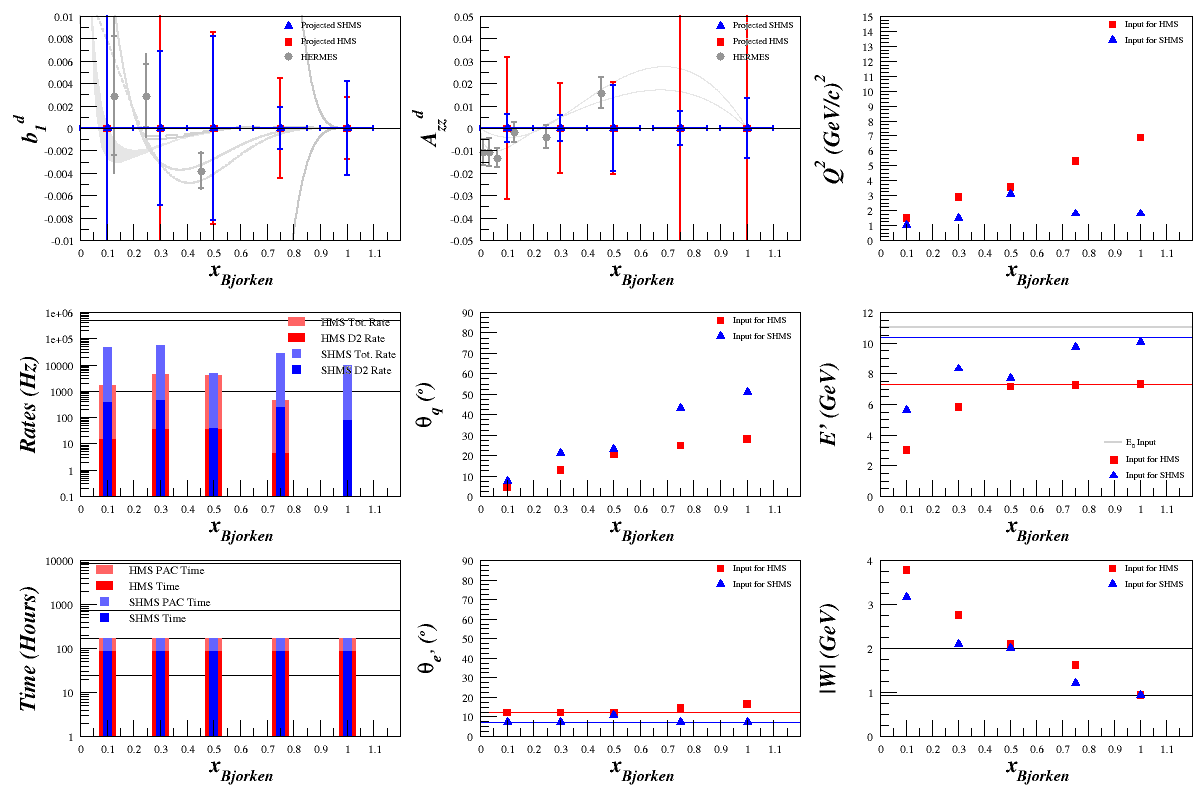
Some of the above still needs to be implemented, namely finding "sweet spots" in F₁, but without that our statistics currently look like:

→ The error bars are calculated from:

$dA_{zz} = \left( \frac{2}{f_{\mathrm{dil}}P_{zz}} \right) \cdot \left( \frac{1}{\sqrt{t\cdot R_{\mathrm{Total}}}} \right)$

$db_1^d = |1.5\cdot dA_{zz}| \cdot F_1^d$

--E. Long 18:56, 29 April 2013 (UTC)