Difference between revisions of "Elong-15-04-30"
(→T20) |
|||
| Line 27: | Line 27: | ||
<math>\sigma_{elastic} = \sigma_{Mott} \left[ A + B \tan^2 \left( \frac{\theta}{2} \right) \right]\delta(E'-E'_{el})</math> | <math>\sigma_{elastic} = \sigma_{Mott} \left[ A + B \tan^2 \left( \frac{\theta}{2} \right) \right]\delta(E'-E'_{el})</math> | ||
| − | behaves as expected. | + | behaves as expected. I can also "smear" the elastic peak more with smaller n, but since the code integrates over the area it should be fine either way. |
{| border="1" style="text-align:center;" | {| border="1" style="text-align:center;" | ||
Revision as of 13:08, 30 April 2015
Background
As mentioned previously, I was able to calculate the elastic cross section using a parameterization of the deuteron's elastic form factors. With the A and B form factors, the cross section was estimated as
<math>\sigma = \sigma_{Mott} \left[ A + B \tan^2 \left( \frac{\theta}{2} \right) \right]</math>
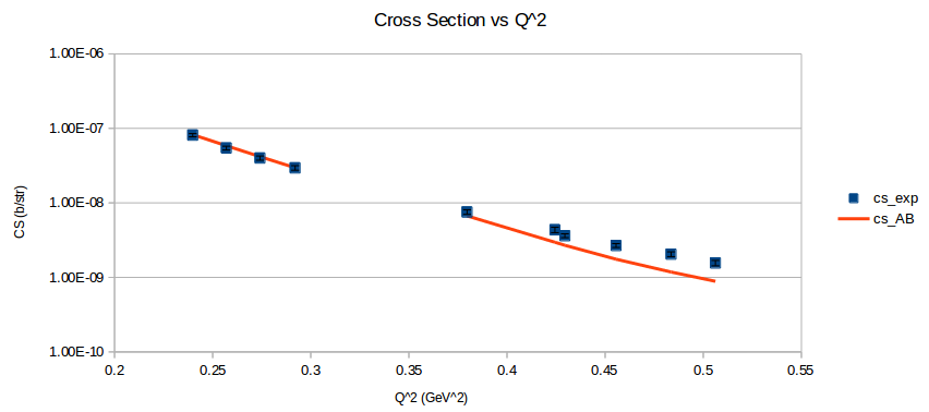
I found a paper from Galster (1971) that included elastic cross sections (and not just A and B), which I was able to reproduce well. (Note: The dip around Q2=0.5 is because of the parameterization underestimating A.)
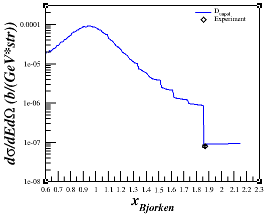
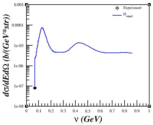
However, when I would plot it versus x or nu,
I wasn't getting what I was expecting in relation to the QE peak.
The Fix
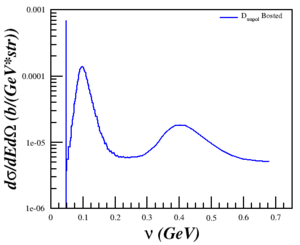
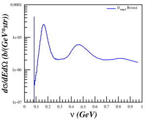
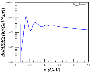
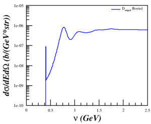
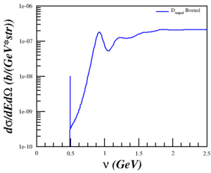
Discussing the issue with Doug and Donal, I realized that the problem was that I was trying to compare a single-derivative elastic cross section with a double-derivative QE cross section, so what I was plotting was the area of the elastic peak and not the peak itself. This was fixed by using a delta function, estimated as <math>\delta(E'-E'_{el}) \approx \frac{n}{\sqrt{\pi}}e^{-n^2 (E'-E'_{el})^2}</math> with <math>n = 5000</math> and <math>E'_{el}=\frac{Q^2}{(2M_D)}</math>, to the cross section. Now, the cross section is calculated by
<math>\sigma = \sigma_{Bosted} + \sigma_{elastic}</math>
where
<math>\sigma_{elastic} = \sigma_{Mott} \left[ A + B \tan^2 \left( \frac{\theta}{2} \right) \right]\delta(E'-E'_{el})</math>
behaves as expected. I can also "smear" the elastic peak more with smaller n, but since the code integrates over the area it should be fine either way.
| <math>Q^2 = 0.18</math> (GeV2) | <math>Q^2 = 0.31</math> (GeV2) | <math>Q^2 = 0.71</math> (GeV2) | <math>Q^2 = 1.50</math> (GeV2) | <math>Q^2 = 1.80</math> (GeV2) |
|---|---|---|---|---|
 |
 |
 |
 |
|
The Rates
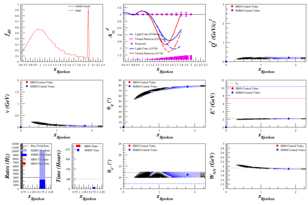
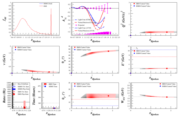
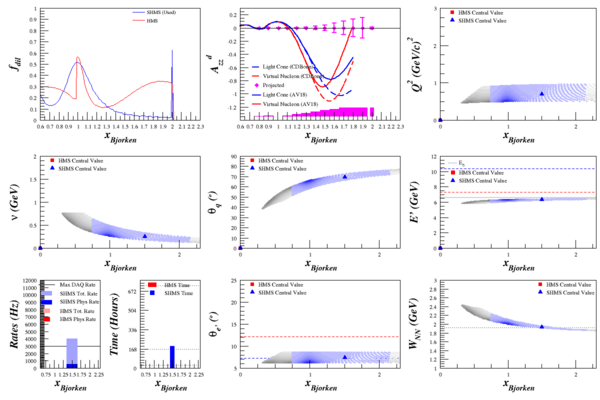
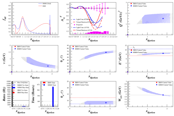
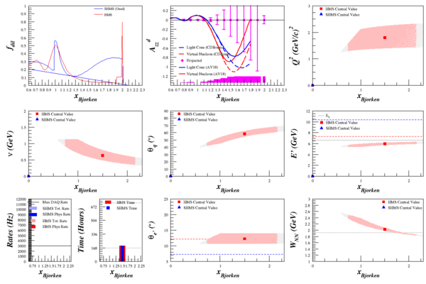
My rates code requires double-derivative <math>\frac{d^2\sigma}{d\Omega dE'}</math> cross section to work, as it algebraically integrates over small bins in <math>\Omega</math> and <math>E'</math>. Running this through the rates code allowed me to calculate elastic <math>A_{zz}</math>, which has significantly smaller uncertainty from its QE neighbors due to the spike in the dilution factor.
Note1: Ignore the LC and VN curves on all but the E=8.8 GeV plots. I was interested just in x=2 for the moment, and lazily didn't remove them.
Note2: For E=8.8 GeV, ignore the x<2 QE Azz uncertainties. It uses the Bosted model, because the elastic calculations didn't play nice next to Misak's model. If you remember, Misak's model gives us a more accurate dilution factor in this region.
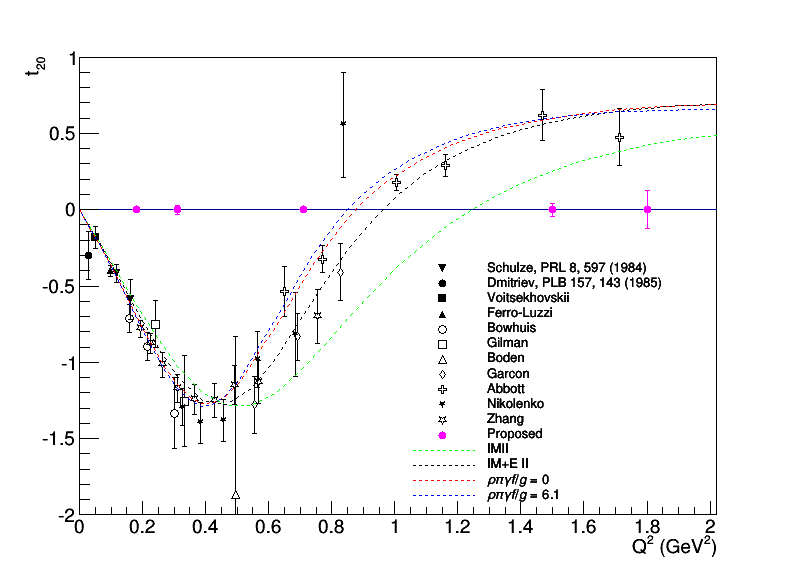
<math>T_{20}</math>
With all of this, I can now calculate the statistical uncertainty we expect for <math>T_{20}</math>.
